Which among the busiest air routes in Europe could actually be travelled by land?

Even just considering only air routes with more than 500 000 passengers per year, 75 million passengers a year could get to their destination in less than six hours by train

Introduction

This document outlines the process of getting data about flights in Europe and matching them with a dataset recently produced by OBC Transeuropa for Greenpeace that includes details about train travel on the busiest of those routes.

The process seems straightforward, given that Eurostat distributes a number of datasets with flight data, but as will be apparent, there are a number of intermediate steps needed to clean and standardise the data.

These include:

• deal with inconsistencies in the original datasets (missing data, non-standard codes, flights to “unknown airports”, to oil rigs, etc.)
• deal with the fact that in some instances more than one airport serve the same city, and within the scope of this analysis all airports serving a given city should really be the same route
• merge data so that routes in both directions are counted as the same
• define which routes cannot possibly be travelled by train (as source or destination are on an island, or exceedingly distant)
• find coordinates of airports and their relative city hubs for visualisation and getting data about distance
• match the result with the above-mentioned train datasets

In the process, a considerable number of intermediate datasets have been generated. You can find some details about them, including a download link, in the final section of this document.

Starting question and operationalisation

What are the main routes in Europe that are currently travelled by flight but could instead be travelled by train?

1. We need a dataset with the number of passengers across all main flight routes in Europe

2. We merge routes serving different airports associated to the same city, as the alternative train route would supposedly be more or less the same; if we have to choose a starting point for a land route for people travelling from Luton airport in the UK, we take London, not Luton.

3. We exclude routes with no land/plausible train connection between them, e.g. flights to and from islands that have no train connection. As a result, for example, flights to and from the UK and the European mainland are included (there is a train connection), while all flights from Ireland to the European mainland are excluded. To clarify: flights within Ireland (e.g. Dublin to Cork) would be included by this rule (in practice, no route within islands unconnected to the European mainland is a major European route).

4. We exclude those routes that cannot be reasonably travelled by land or that would take huge amounts of time, and focus only on the main routes for clarity of analysis. To limit the scope of analysis, the train dataset produced by OBC Transeuropa for Greenpeace takes Eurocontrol’s definition of “short haul” flight, i.e. all those flights shorter than 1500 km, and keeps only the corresponding routes. In this document, no hard limit is set, but the distance for each route is included in the exported datasets.

Key data sources used in the process are the avia_par_ datasets distributed by Eurostat and Wikidata (accessed via the tidywikidatar package created for EDJNet).

The avia_par_ datasets

Eurostat distributes a series of datasets with details of the number of passengers flying to and from European airports. There is not a unified European dataset, but rather one per country. “avia_par_” (followed by a country code).

Here are some basic information about data availability:

fs::dir_create("data")
avia_par_search_file <- fs::path("data", "avia_par_search.csv")

if (fs::file_exists(avia_par_search_file)) {
  avia_par_search_df <- readr::read_csv(file = avia_par_search_file, show_col_types = FALSE)
} else {
  avia_par_search_df <- eurostat::search_eurostat("Air passenger transport between the main airports of")
  readr::write_csv(x = avia_par_search_df, file = avia_par_search_file)
}

avia_par_search_df %>%
  dplyr::mutate(title = stringr::str_remove(title, "Air passenger transport between the main airports of ") %>%
    stringr::str_remove("and their main partner airports \\(routes data\\)")) %>%
  reactable::reactable(filterable = TRUE, sortable = TRUE, resizable = TRUE)

To process the data further it is necessary to combine the datasets and make some choices about which data to keep.

In further steps we will:

• keep only data for 2019 (last pre-pandemic year)
• keep only yearly data (more granular data are available for at least some countries)
• keep only data involving European airports included in the datasets (this means, e.g. removing oversea flights such as those to New York)
• use passengers (“PAS”) as the unit of analysis (not “seats”, or “flights”, which would also be available)
• use “passengers carried (departures)”; only departures rather than totals (departure plus arrivals) to prevent double counting, and “passengers carried” (rather than the slightly different “passengers on board”).

Having data about 35 European countries, this approach means we should complete data about all flights departing from these these countries.

avia_par_PAS_CRD_DEP_file <- fs::path("data", "avia_par_PAS_CRD_DEP_df.csv")

if (fs::file_exists(avia_par_PAS_CRD_DEP_file)) {
  avia_par_PAS_CRD_DEP_df <- readr::read_csv(file = avia_par_PAS_CRD_DEP_file)
} else {
  avia_par_PAS_CRD_DEP_df <- purrr::map_dfr(
    .x = avia_par_search_df$code,
    .f = function(current_code) {
      eurostat::get_eurostat(
        id = current_code,
        time_format = "num", # year as numeric
        select_time = "Y", # yearly data (quarterly and monthly may be available)
        filters = list(
          time = 2019 # only 2019
        )
      ) %>%
        dplyr::mutate(source = current_code) %>%
        dplyr::filter(
          is.na(values) == FALSE, # drop row when data not available
          unit == "PAS", # passengers as unit (not seats or flights
          tra_meas == "PAS_CRD_DEP" # passengers carried departures (to prevent double counting)
        )
    }
  )

  readr::write_csv(
    x = avia_par_PAS_CRD_DEP_df,
    file = avia_par_PAS_CRD_DEP_file
  )
}

if (fs::file_exists(path = fs::path("data", "airp_pr_codes.csv"))) {
  airp_pr_codes_df <- readr::read_csv(file = fs::path("data", "airp_pr_codes.csv"))
} else {
  airp_pr_codes_df <- eurostat::get_eurostat_dic(dictname = "airp_pr")
  readr::write_csv(x = airp_pr_codes_df, file = fs::path("data", "airp_pr_codes.csv"))
}

Here and elsewhere, this document includes some automatic checks to ensure no obvious issues emerge during data processing.

library("testthat")
testthat::test_that(
  desc = "Only one unit/indicator/timeframe is kept, no double counting",
  code = {
    expect_equal(
      object = avia_par_PAS_CRD_DEP_df %>%
        dplyr::distinct(unit) %>%
        nrow(),
      expected = 1
    )

    expect_equal(
      object = avia_par_PAS_CRD_DEP_df %>%
        dplyr::distinct(tra_meas) %>%
        nrow(),
      expected = 1
    )

    expect_equal(
      object = avia_par_PAS_CRD_DEP_df %>%
        dplyr::distinct(time) %>%
        nrow(),
      expected = 1
    )
  }
)

Test passed 😀

# retrieving arrivals for further checks, even if focusing on departures
avia_par_PAS_CRD_ARR_file <- fs::path("data", "avia_par_PAS_CRD_ARR_df.csv")

if (fs::file_exists(avia_par_PAS_CRD_ARR_file)) {
  avia_par_PAS_CRD_ARR_df <- readr::read_csv(file = avia_par_PAS_CRD_ARR_file)
} else {
  avia_par_PAS_CRD_ARR_df <- purrr::map_dfr(
    .x = avia_par_search_df$code,
    .f = function(current_code) {
      eurostat::get_eurostat(
        id = current_code,
        time_format = "num", # year as numeric
        select_time = "Y", # yearly data (quarterly and monthly may be available)
        filters = list(
          time = 2019 # only 2019
        )
      ) %>%
        dplyr::mutate(source = current_code) %>%
        dplyr::filter(
          is.na(values) == FALSE, # drop row when data not available
          unit == "PAS", # passengers as unit (not seats or flights
          tra_meas == "PAS_CRD_ARR" # passengers carried arrivals (to prevent double counting)
        )
    }
  )

  readr::write_csv(
    x = avia_par_PAS_CRD_ARR_df,
    file = avia_par_PAS_CRD_ARR_file
  )
}

The Eurostat dataset looks as follows, showing data for all flights departing from an airport included in this dataset. It is important to highlight that at this stage this is a rather strange datasets, as it includes flights both from and to European destinations (e.g. taking data on London to Amsterdam from the UK dataset, and Amsterdam to London in the UK dataset), but only departures from flights to non-European destinations (e.g. flights London to New York are included, but New York to London aren’t). Routes are defined by a string composed of: departure_country_code_departure_ICAO_airport_code_arrival_country_code_arrival_ICAO_airport_code

avia_par_PAS_CRD_DEP_df %>%
  reactable::reactable(filterable = TRUE, sortable = TRUE, resizable = TRUE)

.csv file: avia_par_PAS_CRD_DEP_df.csv

Let’s have a look at some summary statistics.

How many routes and passengers appear in the dataset for each country?

avia_par_PAS_CRD_DEP_df %>%
  dplyr::group_by(source, .drop = TRUE) %>%
  dplyr::summarise(
    routes_per_country = dplyr::n(),
    total_passengers = sum(values)
  ) %>%
  reactable::reactable(filterable = TRUE, sortable = TRUE, resizable = TRUE, 
                       columns = list(total_passengers = reactable::colDef(format = reactable::colFormat(
      separators = TRUE,
      digits = 0
    ))))

routes_passengers_scatter_gg <- avia_par_PAS_CRD_DEP_df %>%
  dplyr::group_by(source, .drop = TRUE) %>%
  dplyr::summarise(
    routes_per_country = dplyr::n(),
    total_passengers = sum(values)
  ) %>%
  dplyr::mutate(country = stringr::str_extract(source, "[a-z][a-z]$") %>% stringr::str_to_upper()) %>%
  ggplot2::ggplot(mapping = ggplot2::aes(x = total_passengers, y = routes_per_country)) +
  ggplot2::geom_point() +
  ggplot2::scale_y_continuous(name = "Number of routes") +
  ggplot2::scale_x_continuous(name = "Number of departing passengers", labels = scales::number) +
  theme_minimal()


ggiraph::girafe(code = print(routes_passengers_scatter_gg +
  ggiraph::geom_point_interactive(aes(tooltip = country), size = 2)))

N.B. see which country is which by hovering the graph

At first glance there is no major outlier or piece of data that is self-evidently wrong, but we notice that there are data only from 34 countries, even if the original dataset is available for 35: Turkey is missing.

european_countries_df <- avia_par_PAS_CRD_DEP_df %>%
  dplyr::distinct(source) %>%
  dplyr::transmute(country_code = stringr::str_extract(source, "[a-z][a-z]$") %>% stringr::str_to_upper())

european_countries_df %>%
  reactable::reactable(sortable = TRUE)

As it turns out, this is due to the fact that the dataset for Turkey, avia_par_tr, does not include data for “passengers on board” (PAS_BRD) but not for “passengers carried” (PAS_CRD).

Plotting the 34 countries currently included on a map, we notice that Bosnia and Albania are not included. Pristina airport is inconsistently found among destinations but never as departure. ¹. Ercan airport in Northern Cyprus is similarly not included.

world_sf_file <- fs::path("data", "world_geo_data", "world_sf.rds")

if (fs::file_exists(world_sf_file)) {
  world_sf <- readr::read_rds(world_sf_file)
} else {
  fs::dir_create(fs::path("data", "world_geo_data"))
  download.file(
    url = "https://gisco-services.ec.europa.eu/distribution/v2/countries/download/ref-countries-2020-60m.geojson.zip",
    destfile = fs::path("data", "world_geo_data", "world.geojson.zip")
  )

  unzip(fs::path("data", "world_geo_data", "world.geojson.zip"),
    exdir = fs::path("data", "world_geo_data")
  )

  world_sf <- sf::st_read(dsn = fs::path("data", "world_geo_data", "CNTR_RG_60M_2020_4326.geojson"))

  saveRDS(object = world_sf, file = fs::path("data", "world_geo_data", "world_sf.rds"))
}



ggplot2::ggplot() +
  ggplot2::geom_sf(data = world_sf, fill = "lightgrey") +
  ggplot2::geom_sf(
    data = dplyr::left_join(
      x = european_countries_df,
      y = world_sf %>% dplyr::rename(country_code = CNTR_ID),
      by = "country_code"
    ) %>%
      sf::st_as_sf(),
    fill = "lightgreen"
  ) +
  ggplot2::scale_x_continuous(limits = c(-30, 50)) +
  ggplot2::scale_y_continuous(limits = c(35, 72)) +
  ggplot2::theme_minimal()

If we dismiss domestic flights, in principle we could still obtain the relevant data for flights involving European airports included in the dataset, by, for example, adding separately all flights to Bosnia recorded as departures, and all flights from Bosnia recorded in arrivals. We could also include Turkey, based on the rather similar “passengers on board indicator”.

avia_par_tr_PAS_BRD_DEP_file <- fs::path("data", "avia_par_tr_PAS_BRD_DEP.csv")

if (fs::file_exists(avia_par_tr_PAS_BRD_DEP_file)==FALSE) {
  avia_par_tr_PAS_BRD_DEP_df <- eurostat::get_eurostat(
        id = "avia_par_tr",
        time_format = "num", # year as numeric
        select_time = "Y", # yearly data (quarterly and monthly may be available)
        filters = list(
          time = 2019 # only 2019
        )
      ) %>%
        dplyr::mutate(source = "avia_par_tr") %>%
        dplyr::filter(
          is.na(values) == FALSE, # drop row when data not available
          unit == "PAS", # passengers as unit (not seats or flights
          tra_meas == "PAS_BRD_DEP" # passengers carried departures (to prevent double counting)
        )
} else {
  avia_par_tr_PAS_BRD_DEP_df <- readr::read_csv(avia_par_tr_PAS_BRD_DEP_file)
}

Add missing countries and deal with inconsistent data from Czechia

Conceptually, we expect all routes to be travelled in both directions. This is probably the case, but is not fully reflected in the dataset. In particular, data on departure from Czechia include only the country of destination, not the specific airport.

avia_par_PAS_CRD_DEP_df %>%
  filter(source == "avia_par_cz") %>%
  rename(route_code = airp_pr) %>%
  left_join(y = airp_pr_codes_df %>% rename(route_code = code_name), by = "route_code") %>%
  reactable::reactable()

Not all is lost: we can still get all flights from Czechia by taking the dataset on arrivals for all other European countries, which should give the figure we need.

We first remove from the dataset based on departures all routes involving Czechia, then take from the dataset on arrivals all routes as recorded coming from Czechia and merge them.

Since we’re at it, let’s add also countries that are not (yet) included in the dataset, such as Bosnia, Albania, Kosovo, and Moldova.

missing_countries_v <- c("CZ", "BA", "AL", "MD", "XK")

departures_without_cz_df <- avia_par_PAS_CRD_DEP_df %>%
  filter(source != "avia_par_cz")

arrivals_with_missing_df <- avia_par_PAS_CRD_ARR_df %>%
  mutate(destination_country = stringr::str_extract(
    string = airp_pr,
    pattern = "[A-Z]{2}(?=_[[:print:]]{4}$)"
  )) %>%
  filter(destination_country %in% missing_countries_v) %>%
  select(-destination_country)

avia_par_PAS_CRD_fixed_df <- bind_rows(
  departures_without_cz_df,
  arrivals_with_missing_df,
  avia_par_tr_PAS_BRD_DEP_df
) %>%
  group_by(unit, airp_pr, time, source) %>%
  summarise(
    tra_meas = "PAS_CRD_DEP",
    values = sum(values), .groups = "drop"
  ) %>%
  ungroup() %>%
  select(unit, tra_meas, airp_pr, time, values, source)


if (fs::file_exists(fs::path("data", "avia_par_PAS_CRD_fixed.csv")) == FALSE) {
  readr::write_csv(
    x = avia_par_PAS_CRD_fixed_df,
    file = fs::path("data", "avia_par_PAS_CRD_fixed.csv")
  )
}

avia_par_PAS_CRD_fixed_df %>%
  reactable(filterable = TRUE, sortable = TRUE)

.csv file: avia_par_PAS_CRD_fixed.csv

So we should have now data about flights to and from these countries. For the countries in yellow there are some more inconsistencies: in particular, only flights to European airports are effectively included and flights among them would not appear.

ggplot2::ggplot() +
  ggplot2::geom_sf(data = world_sf, fill = "lightgrey") +
  ggplot2::geom_sf(
    data = dplyr::left_join(
      x = european_countries_df,
      y = world_sf %>% dplyr::rename(country_code = CNTR_ID),
      by = "country_code"
    ) %>%
      sf::st_as_sf(),
    fill = "lightgreen"
  ) +
    ggplot2::geom_sf(
    data = dplyr::left_join(
      x = tibble::tibble(country_code = c(missing_countries_v)),
      y = world_sf %>% dplyr::rename(country_code = CNTR_ID),
      by = "country_code"
    ) %>%
      sf::st_as_sf(),
    fill = "gold"
  ) +
  ggplot2::scale_x_continuous(limits = c(-30, 50)) +
  ggplot2::scale_y_continuous(limits = c(35, 72)) +
  ggplot2::theme_minimal()

Transforming codes into routes

Now that we have a better picture of the scope of the dataset, we can find and use the relevant dictionary to turn airport route codes into more human-readable labels:

airp_pr_codes_df %>%
  reactable::reactable(filterable = TRUE)

.csv file: airp_pr_codes.csv

We also create a more polished version where each airport has its country, code, and name in separate columns.

It appears that occasionally airports located in Serbia, Montenegro, and Kosovo, rather than having the conventional two-letter country code, are marked as “RS_ME”, which is a 5 character string. We’ll fix them manually.

airp_pr_codes_sep_pre_df <- airp_pr_codes_df %>%
  mutate(code_name = stringr::str_replace(code_name, "_RS_ME_LYPR", "_XK_LYPR")) %>% # set pristina to XK
  mutate(code_name = stringr::str_replace(code_name, "_RS_ME_LY99", "_RS_LY99")) %>% # set generic RS_ME to RS 
  # (anyway, removed in following step, as these are "unknown")
  mutate(code_name = stringr::str_replace(code_name, "_RS_ME_LYBE", "_RS_LYBE")) %>% # set Belgrade to RS
  mutate(code_name = stringr::str_replace(code_name, "_RS_ME_LYTI", "_ME_LYTI")) %>% # set Podgorica to ME
  mutate(code_name = stringr::str_replace(code_name, "_RS_ME_LYPG", "_ME_LYPG")) %>% # set Podgorica to ME
  mutate(code_name = stringr::str_replace(code_name, "_RS_ME_LYNI", "_RS_LYNI")) %>% # set Nis to RS
  tidyr::separate(
    col = code_name,
    into = c(
      "origin_country",
      "origin_airport",
      "destination_country",
      "destination_airport"
    ),
    sep = "_",
    remove = TRUE
  ) %>%
  #  filter(origin_country %in% european_countries_df$country_code|destination_country %in% european_countries_df$country_code) %>%
  mutate(origin_airport_name = stringr::str_extract(string = full_name, pattern = "^.*(?=airport - )") %>%
    stringr::str_remove(" airport.*") %>%
    stringr::str_squish()) %>%
  mutate(destination_airport_name = stringr::str_extract(string = full_name, pattern = "(?=airport - ).*") %>%
    stringr::str_remove_all("airport") %>%
    stringr::str_remove(" - ") %>%
    stringr::str_squish())

airp_pr_codes_clean_df <- bind_rows(
  airp_pr_codes_sep_pre_df %>% transmute(
    country = origin_country,
    airport_code = origin_airport,
    airport_name = origin_airport_name
  ),
  airp_pr_codes_sep_pre_df %>% transmute(
    country = destination_country,
    airport_code = destination_airport,
    airport_name = destination_airport_name
  )
) %>%
  dplyr::distinct() %>%
  # filter(is.na(airport_name)==FALSE,
  #        stringr::str_detect(airport_code, "99", negate = TRUE),
  #        stringr::str_detect(airport_code, "00", negate = TRUE),
  #        airport_name != "Unknown") %>%
  distinct(airport_code, .keep_all = TRUE) %>%
  dplyr::arrange(country, airport_name)


if (fs::file_exists(fs::path("data", "airp_pr_codes_clean.csv")) == FALSE) {
  readr::write_csv(airp_pr_codes_clean_df, file = fs::path("data", "airp_pr_codes_clean.csv"))
}

airp_pr_codes_clean_df %>%
  reactable::reactable(filterable = TRUE, sortable = TRUE, resizable = TRUE)

.csv file: airp_pr_codes_clean.csv

Merging the two datasets, and putting this in order for the most popular routes, we obtain the following:

routes_dep_label_df <- avia_par_PAS_CRD_fixed_df %>%
  dplyr::transmute(route_code = airp_pr, pas_crd_dep = values) %>%
  dplyr::left_join(
    y = airp_pr_codes_df %>% dplyr::rename(route_code = code_name, route_name = full_name),
    by = "route_code"
  ) %>%
  dplyr::select(route_code, route_name, pas_crd_dep) %>%
  dplyr::arrange(dplyr::desc(pas_crd_dep))

routes_dep_label_df %>%
  reactable::reactable(
    filterable = TRUE, sortable = TRUE, resizable = TRUE, 
    columns = list(pas_crd_dep = reactable::colDef(format = reactable::colFormat(
      separators = TRUE,
      digits = 0
    ))))

testthat::test_that(
  desc = "Matching of labels leaves no rows unlabelled",
  code = {
    expect_equal(
      object = routes_dep_label_df %>%
        dplyr::filter(is.na(route_name)) %>%
        nrow(),
      expected = 0
    )
  }
)

Test passed 😀

We notice that some airport codes including double-zero or double-nine (00 or 99) are actually generic codes for “unknown airport in given country”.

Beyond Czechia, which other “unknown airports” appear in the dataset?

avia_par_PAS_CRD_fixed_labelled_df <- avia_par_PAS_CRD_fixed_df %>%
  rename(route_code = airp_pr) %>%
  left_join(y = routes_dep_label_df, by = "route_code") %>%
  transmute(route_code,
    route_name,
    passengers = values
  )

if (fs::file_exists(fs::path("data", "avia_par_PAS_CRD_fixed_labelled.csv")) == FALSE) {
  readr::write_csv(x = avia_par_PAS_CRD_fixed_labelled_df, file = fs::path("data", "avia_par_PAS_CRD_fixed_labelled.csv"))
}

avia_par_PAS_CRD_fixed_labelled_df %>%
  reactable::reactable(sortable = TRUE, resizable = TRUE, filterable = TRUE, 
                       columns = list(passengers = reactable::colDef(format = reactable::colFormat(
      separators = TRUE,
      digits = 0
    )))
                       )

.csv file: avia_par_PAS_CRD_DEP_labelled.csv

avia_par_PAS_CRD_fixed_labelled_df %>%
  dplyr::filter(
    stringr::str_detect(string = route_name, pattern = stringr::regex("unknown", ignore_case = TRUE)),
    stringr::str_detect(string = route_code, pattern = "^CZ_", negate = TRUE)
  ) %>%
  arrange(desc(passengers)) %>%
  reactable::reactable()

Somewhat puzzlingly, there are hundreds of thousands of passengers who, according to official data, flew into the unknown taking off from major European airports, mostly from either Brussels or Turkish airports. There is seemingly little we can do to recover those data from the available dataset.

Even besides this, this dataset is however a mess, as it counts travels for both ways for intra-European flights but only one way for extra-European flights. Having only departures, it has for example flights from London to New York, but not from New York to London. However, it has both flights from London to Paris as well as those from Paris to London, the former taken from the avia_par_uk dataset, the latter from the avia_par_fr dataset.

To get a more meaningful and consistent dataset we should filter the data and keep only routes involving European countries. Besides, we are interested in the total traffic on a route, so that, for example London-Paris and Paris-London passengers are summed together.

First, let’s remove all flights involving a non-European airport (to be more precise, an airport that is not located in one of the countries we know are included in the dataset).

So we take it again from the original codes and break out the airport codes:

avia_par_PAS_CRD_fixed_sep_df <- avia_par_PAS_CRD_fixed_df %>%
  dplyr::select(airp_pr, values) %>%
  tidyr::separate(
    col = airp_pr,
    into = c(
      "origin_country",
      "origin_airport",
      "destination_country",
      "destination_airport"
    ),
    sep = "_",
    remove = TRUE
  ) %>%
  dplyr::rename(passengers = values)

avia_par_PAS_CRD_fixed_sep_df %>%
  reactable::reactable(
    filterable = TRUE,
    sortable = TRUE,
    columns = list(passengers = reactable::colDef(format = reactable::colFormat(
      separators = TRUE,
      digits = 0
    )))
  )

We can then keep in the “destination_country” column only countries that are present in the “origin_country” column, making sure to keep Czechia.

avia_par_PAS_CRD_fixed_sep_european_df <- avia_par_PAS_CRD_fixed_sep_df %>%
  filter(destination_country %in% unique(c(missing_countries_v, origin_country)))

# not so relevant after Czechia fix
test_that(desc = "origin countries plus missing countries and destination countries are the same", code = {
  expect_equal(
    object = avia_par_PAS_CRD_fixed_sep_european_df %>%
      distinct(origin_country) %>%
      arrange(origin_country) %>%
      pull(origin_country) %>%
      c(., missing_countries_v) %>%
      sort(),
    expected = avia_par_PAS_CRD_fixed_sep_european_df %>%
      distinct(destination_country) %>%
      arrange(destination_country) %>%
      pull(destination_country)
  )
})

Test passed 🎉

We can now add together passengers from both directions of the flight, and have a first ranking of the top European routes included in the dataset. The order of airports within a route is determined by the alphabetical order of the airport code (so, for example, it’s Barcelona-Madrid and not vice-versa because Barcelona’s airport code - ES_LEBL - alphabetically precedes Madrid’s code ES_LEMD). For consistency, this is applied also to the rare cases where only the route in the inverse direction is effectively included in the original dataset. Flights to “unknown airports”are also removed.

There’s also a big question about what to do with data from Turkey, which has a lot of busy air routes, many of them domestic. Given that the focus is train routes across the European Union, we’ll leave Turkey out of the main analysis, even if some of the busiest domestic routes in Turkey would be clearly good candidates for a train alternative (e.g. the 2.75 million passengers flying between Istanbul and Izmir.)

european_routes_ranking_alf_df <- avia_par_PAS_CRD_fixed_sep_european_df %>%
  tidyr::unite(col = "origin_airport", dplyr::contains("origin_"), sep = "_") %>%
  tidyr::unite(col = "destination_airport", dplyr::contains("destination_"), sep = "_") %>%
  dplyr::mutate(combo_id = row_number()) %>%
  tidyr::pivot_longer(
    cols = c(
      "origin_airport",
      "destination_airport"
    ),
    names_to = "type",
    values_to = "airport"
  ) %>%
  dplyr::group_by(combo_id) %>%
  dplyr::arrange(airport) %>%
  dplyr::summarise(
    passengers = unique(passengers),
    airport = paste(airport, collapse = "_")
  ) %>%
  dplyr::group_by(airport) %>%
  dplyr::summarise(passengers = sum(passengers)) %>%
  dplyr::transmute(route_code = airport, passengers) %>%
  dplyr::arrange(dplyr::desc(passengers)) %>%
  dplyr::mutate(ranking = dplyr::row_number()) %>%
  left_join(
    y = airp_pr_codes_df %>%
      dplyr::rename(route_code = code_name, route_name = full_name),
    by = "route_code"
  ) %>%
  transmute(ranking, route_code, route_name, passengers) %>%
  mutate(
    country1 = stringr::str_extract(route_code, pattern = "[A-Z][A-Z]"),
    country2 = stringr::str_extract(route_code, pattern = "_[A-Z][A-Z]_") %>% stringr::str_remove_all("_")
  ) %>%
  mutate(type = dplyr::if_else(country1 == country2, "domestic", "international")) %>%
  tidyr::unite(col = "country", country1, country2, sep = "_", remove = TRUE)
# dplyr::filter(stringr::str_detect(string = route_name,
#                                   pattern = stringr::regex("Unknown", ignore_case = TRUE), negate = TRUE))


route_names_fix_df <- european_routes_ranking_alf_df %>%
  transmute(ranking,
    route_code,
    route_code_reverse = stringr::str_c(
      stringr::str_extract(route_code, "[A-Z]{2}_[[:alnum:]]{4}$"),
      "_",
      stringr::str_extract(route_code, "^[A-Z]{2}_[[:alnum:]]{4}")
    )
  ) %>%
  left_join(
    y = airp_pr_codes_df %>%
      dplyr::rename(route_code = code_name, route_name = full_name),
    by = "route_code"
  ) %>%
  left_join(
    y = airp_pr_codes_df %>%
      dplyr::rename(
        route_code_reverse = code_name,
        route_name_reverse = full_name
      ),
    by = "route_code_reverse"
  ) %>%
  transmute(
    ranking,
    route_name = dplyr::if_else(is.na(route_name),
      stringr::str_c(
        stringr::str_extract(route_name_reverse, " - [[:print:]]+$") %>%
          stringr::str_remove(" - "),
        " - ",
        stringr::str_extract(route_name_reverse, "^[[:print:]]+ - ") %>%
          stringr::str_remove(" - ")
      ),
      route_name
    )
  )



# which(european_routes_ranking_alf_df$route_name[is.na(european_routes_ranking_alf_df$route_name)])
#
# european_routes_ranking_alf_df$route_name[is.na(european_routes_ranking_alf_df$route_name)] <-
# european_routes_ranking_revalf_df$route_name[is.na(european_routes_ranking_alf_df$route_name)]


european_routes_ranking_with_turkey_df <- european_routes_ranking_alf_df %>%
  select(-route_name) %>%
  left_join(route_names_fix_df, by = "ranking") %>%
  mutate(
    origin_airport_code = stringr::str_extract(route_code, "^[A-Z]{2}_[[:alnum:]]{4}"),
    destination_airport_code = stringr::str_extract(route_code, "[A-Z]{2}_[[:alnum:]]{4}$"),
    origin_airport_name = stringr::str_extract(route_name, "^[[:print:]]+ - ") %>%
      stringr::str_remove(" - "),
    destination_airport_name = stringr::str_extract(route_name, " - [[:print:]]+$") %>%
      stringr::str_remove(" - ")
  ) %>%
  mutate(
    origin_airport_country = stringr::str_extract(origin_airport_code, "^[A-Z]{2}"),
    destination_airport_country = stringr::str_extract(destination_airport_code, "^[A-Z]{2}"),
    origin_airport_icao = stringr::str_remove(origin_airport_code, "^[A-Z]{2}_"),
    destination_airport_icao = stringr::str_remove(destination_airport_code, "^[A-Z]{2}_")
  ) %>%
  select(
    ranking,
    type,
    route_code,
    passengers,
    route_name,
    origin_airport_code,
    origin_airport_country,
    origin_airport_icao,
    origin_airport_name,
    destination_airport_code,
    destination_airport_country,
    destination_airport_icao,
    destination_airport_name
  )

european_routes_ranking_df <- european_routes_ranking_with_turkey_df %>% 
  filter(origin_airport_country!="TR", destination_airport_country!="TR") %>% 
  mutate(ranking = row_number())


european_routes_ranking_file <- fs::path(
  "data",
  "european_routes_ranking.csv"
)

if (fs::file_exists(european_routes_ranking_file) == FALSE) {
  readr::write_csv(x = european_routes_ranking_df,
                   file = european_routes_ranking_file)
  
    readr::write_csv(x = european_routes_ranking_with_turkey_df,
                   file = fs::path(
  "data",
  "european_routes_ranking_with_turkey.csv"
))
  
}

Data including Turkey:

european_routes_ranking_with_turkey_df %>%
  reactable::reactable(
    filterable = TRUE,
    sortable = TRUE,
    columns = list(passengers = reactable::colDef(format = reactable::colFormat(
      separators = TRUE,
      digits = 0
    )))
  )

.csv file: european_routes_ranking_with_turkey.csv

Data not including Turkey:

european_routes_ranking_df %>%
  reactable::reactable(
    filterable = TRUE,
    sortable = TRUE,
    resizable = TRUE, 
    columns = list(passengers = reactable::colDef(format = reactable::colFormat(
      separators = TRUE,
      digits = 0
    )))
  )

.csv file: european_routes_ranking.csv

Notice that this table includes routes between specific airports, not between cities. We’ll get to that in a second.

Before moving on, let’s have a quick look at the data we have so far.

european_routes_ranking_scatter_gg <- european_routes_ranking_df %>%
  slice_head(n = 250) %>%
  ggplot(mapping = aes(x = type, y = passengers)) +
  geom_point() +
  scale_y_continuous(
    name = "",
    labels = scales::number, limits = c(0, NA)
  ) +
  scale_x_discrete("") +
  labs(title = "Number of passengers on top 250 European routes") +
  theme_minimal()


ggiraph::girafe(code = print(european_routes_ranking_scatter_gg +
  ggiraph::geom_point_interactive(aes(tooltip = route_name), size = 2)))

Looking at the top routes, we notice that many of the most busy are domestic (hover to see name of the route):

european_routes_ranking_bar_gg <- european_routes_ranking_df %>%
  slice_head(n = 20) %>%
  arrange(desc(passengers)) %>%
  mutate(route_code = forcats::as_factor(route_code)) %>%
  ggplot(mapping = aes(x = route_code, y = passengers, fill = type)) +
  geom_col() +
  scale_y_continuous(
    name = "",
    labels = scales::number,
    limits = c(0, NA)
  ) +
  scale_x_discrete("", labels = rep("", 20)) +
  labs(title = "Number of passengers on top 20 European routes") +
  theme_minimal() +
  theme(legend.title = element_blank(), legend.position = "bottom")


ggiraph::girafe(code = print(european_routes_ranking_bar_gg +
  ggiraph::geom_col_interactive(aes(tooltip = route_name))))

Time to move on and filter the data further.

Further oddities in the data

Not yet… :-)

In order to move forward, we must extract the code for each European airport found in the dataset.

origin_airports_df <- avia_par_PAS_CRD_fixed_sep_european_df %>%
  transmute(country = origin_country, airport = origin_airport) %>%
  distinct(country, airport)

destination_airports_df <- avia_par_PAS_CRD_fixed_sep_european_df %>%
  transmute(country = destination_country, airport = destination_airport) %>%
  distinct(country, airport)

In doing so, it emerges that there are some airports that appear only as the destination, and some only as points of departure, which would be highly unusual and most likely points at some inconsistencies in the data.

Airports found in departures, but not in destinations:

origin_airports_df %>%
  anti_join(destination_airports_df, by = "airport") %>%
  rename(airport_code = airport) %>%
  left_join(y = airp_pr_codes_clean_df %>% select(-country), by = "airport_code") %>%
  reactable::reactable(sortable = TRUE, filterable = TRUE)

Airports found as destinations, but not as departures (excluding Czechia and the Balkan countries we added separately):

destination_airports_df %>%
   filter(!country %in% missing_countries_v) %>%
  anti_join(origin_airports_df, by = "airport") %>%
  rename(airport_code = airport) %>%
  left_join(y = airp_pr_codes_clean_df %>% select(-country), by = "airport_code") %>%
  reactable::reactable(sortable = TRUE, filterable = TRUE)

Again, short of assuming that the number of flights departing and arriving in an airport is almost always balanced, there is seemingly not much that we can do to fix this. These are anyway all small airport that would anyway not make it to the “top European routes” that is really the objective of this data processing effort.

all_airports_df <- bind_rows(
  origin_airports_df,
  destination_airports_df
) %>%
  distinct(country, airport) %>%
  arrange(country, airport) %>%
  filter(stringr::str_detect(string = airport, pattern = "99", negate = TRUE))

Getting the coordinates of airports and the main city they serve

The first step that needs to be made in order to apply further filtering criteria is to to find the coordinates for each of these airports.

There are some on-line datasets with some data about airports, see for example - https://ourairports.com/data/airports.csv - but no apparent official, comprehensive, and free list.

fs::dir_create("data")

airport_codes_file <- fs::path("data", "airports.csv")
if (fs::file_exists(fs::path("data", "airports.csv")) == FALSE) {
  download.file(
    url = "https://ourairports.com/data/airports.csv",
    destfile = airport_codes_file
  )
}

airport_codes_df <- readr::read_csv(airport_codes_file)


airport_codes_df$ident[is.na(airport_codes_df$gps_code) == FALSE & airport_codes_df$gps_code == "EPLB"] <- "EPLB" # fix Lublin
airport_codes_df$ident[is.na(airport_codes_df$gps_code) == FALSE & airport_codes_df$gps_code == "LSZM"] <- "LSZM"

A useful source for structured data that have no licensing constraints is Wikidata. We can, for example, ask Wikidata for all items that have data for the ICAO code property (“P239”), which is the four-character code that is mostly used to define airports in this dataset. By using Wikidata, we can get coordinates for the vast majority of these airports, as well as gather some additional structured data about them (it is also possible to query for the specific codes included in our dataset, but I prefer to leave this open-ended, facilitating alternative uses).

Wikidata has also a dedicated property - P931 - to make explicit the fact that an airport is understood to serve a major neighbouring city even if its not located in the relevant municipality (e.g. “London” is the value of property P931 for the Luton airport), which will also be useful later on when we merge multiple airports serving the same cities to gauge total traffic between two hubs. When Wikidata suggests more than one hub, we’ll keep only the first.

While we’re at it, we’ll ask Wikidata for some more details, such as the administrative unit where they are located. We’ll also keep the Wikidata identifiers for reference and further processing.

# data are cached locally, but at first run this may take a few hours
library("tidywikidatar")

tw_enable_cache()
tw_set_cache_folder(path = fs::path(
  fs::path_home_r(),
  "R",
  "tw_data"
))
tw_set_language(language = "en")
tw_create_cache_folder(ask = FALSE)


if (fs::file_exists(fs::path("data", "airport_qid.csv"))) {
  airport_qid_df <- readr::read_csv(fs::path("data", "airport_qid.csv"))
} else {
  api_url <- "https://www.wikidata.org/w/api.php?action=query&list=backlinks&blnamespace=0&bllimit=500&bltitle=Property:P239&format=json"

  base_json <- jsonlite::read_json(api_url)

  continue_check <- base_json %>%
    purrr::pluck("continue", "blcontinue")

  all_jsons <- list()
  page_number <- 1

  all_jsons[[page_number]] <- base_json

  while (is.null(continue_check) == FALSE & page_number < 10000) {
    Sys.sleep(0.1)
    message(page_number)
    page_number <- page_number + 1
    base_json <- jsonlite::read_json(stringr::str_c(
      api_url,
      "&blcontinue=",
      continue_check
    ))

    all_jsons[[page_number]] <- base_json

    continue_check <- base_json %>%
      purrr::pluck("continue", "blcontinue")
  }



  all_pages <- purrr::map(
    .x = all_jsons,
    .f = purrr::pluck, "query", "backlinks"
  ) %>%
    purrr::flatten()

  airport_qid_df <- purrr::map_dfr(
    .x = all_pages,
    .f = function(current_page) {
      tibble::tibble(
        qid = current_page %>%
          purrr::pluck(
            "title"
          )
      )
    }
  )

  readr::write_csv(
    x = airport_qid_df,
    fs::path("data", "airport_qid.csv")
  )
}


#
# airport_qid_icao_df <- airport_qid_df %>%
#   dplyr::pull(qid) %>%
#   tw_get_property(p = "P239")

if (fs::file_exists(fs::path("data", "airport_qid_icao_details.csv"))) {
  airport_qid_icao_details_df <- readr::read_csv(file = fs::path("data", "airport_qid_icao_details.csv"))
} else {
  airport_qid_icao_details_df <- airport_qid_df %>%
    dplyr::transmute(
      airport_qid = qid,
      airport = tw_get_label(qid),
      country_qid = tw_get_property_same_length(qid, p = "P17", only_first = TRUE),
      country = tw_get_property_same_length(qid, p = "P17", only_first = TRUE) %>% tw_get_label(),
      administrative_entity_qid = tw_get_property_same_length(qid, p = "P131", only_first = TRUE),
      administrative_entity = tw_get_property_same_length(qid, p = "P131", only_first = TRUE) %>% tw_get_label(),
      coordinates = tw_get_property_same_length(qid, p = "P625", only_first = TRUE),
      iata_code = tw_get_property_same_length(qid, p = "P238", only_first = TRUE),
      icao_code = tw_get_property_same_length(qid, p = "P239"),
      hub_qid = tw_get_property_same_length(qid, p = "P931", only_first = TRUE),
      hub = tw_get_property_same_length(qid, p = "P931", only_first = TRUE) %>% tw_get_label(),
      hub_coordinates = tw_get_property_same_length(qid, p = "P931", only_first = TRUE) %>%
        tw_get_property_same_length(p = "P625", only_first = TRUE),
      replaced_by_qid = tw_get_property_same_length(id = airport_qid, p = "P1366", only_first = TRUE),
      replaced_by_icao_code = tw_get_property_same_length(id = airport_qid, p = "P1366", only_first = TRUE) %>% tw_get_property_same_length(p = "P239")
    ) %>%
    tidyr::unnest(icao_code) %>%
    dplyr::filter(is.na(icao_code) == FALSE) %>%
    dplyr::filter(icao_code != "NA") %>%
    tidyr::separate(
      col = coordinates,
      into = c("latitude", "longitude"),
      sep = ",",
      remove = TRUE,
      convert = TRUE
    ) %>%
    tidyr::separate(
      col = hub_coordinates,
      into = c(
        "hub_latitude",
        "hub_longitude"
      ),
      sep = ",",
      remove = TRUE,
      convert = TRUE
    )

  readr::write_csv(
    x = airport_qid_icao_details_df,
    file = fs::path("data", "airport_qid_icao_details.csv")
  )
}

airport_qid_icao_details_df %>%
  reactable::reactable(sortable = TRUE, resizable = TRUE, filterable = TRUE)

.csv file: airport_qid_icao_details.csv

N.B. If you use this intermediate dataset, be mindful that there are instances where there are two Wikidata items associated with the same ICAO code; this may be related to potential inaccuracies, but also to instances where, for example, a military airbase is located on the same premises as a civilian airport. See below for an alternative version with only one row per ICAO code.

To prevent further issues when matching with other data sources, we’ll proceed to create an additional dataset where there is one row for each ICAO code and they are never repeated. To decide which Wikidata identifier to keep, we’ll proceed in this order of priority, while making sure to keep one row for each ICAO code:

• airports that have the “replaced_by” field in Wikidata go last
• by longitude (missing coordinates goes last)
• by IATA code (missing IATA code goes last)
• by city hub (missing city hub goes last)
• by airport Wikidata identifier (item added earlier to Wikidata is preferred, as duplicates usually refer to some ancillary base usually added later to Wikidata)

These are all Wikidata items that include reference to the same ICAO code; only the first occurrence is kept in the dataset.

airport_qid_icao_details_df %>%
  group_by(icao_code) %>%
  add_count() %>%
  ungroup() %>%
  mutate(airport_qid_numeric = as.numeric(stringr::str_extract(airport_qid, "[[:digit:]]+"))) %>%
  mutate(replaced_by_qid = tw_get_property_same_length(id = airport_qid, p = "P1366", only_first = TRUE)) %>%
  arrange(
    desc(n),
    icao_code,
    is.na(iata_code),
    desc(is.na(replaced_by_qid)),
    airport_qid_numeric,
    is.na(hub)
  ) %>%
  select(airport_qid, airport, icao_code, iata_code, hub, replaced_by_qid, n) %>%
  filter(n > 1) %>%
  group_by(icao_code) %>%
  mutate(keep = row_number() == 1) %>%
  ungroup() %>%
  reactable::reactable(sortable = TRUE, resizable = TRUE, filterable = TRUE)

airport_qid_unique_icao_details_df <- airport_qid_icao_details_df %>%
  group_by(icao_code) %>%
  add_count() %>%
  ungroup() %>%
  mutate(airport_qid_numeric = as.numeric(stringr::str_extract(airport_qid, "[[:digit:]]+"))) %>%
  mutate(
    replaced_by_qid = tw_get_property_same_length(id = airport_qid, p = "P1366", only_first = TRUE),
    replaced_by_icao_code = tw_get_property_same_length(id = airport_qid, p = "P1366", only_first = TRUE) %>% tw_get_property_same_length(p = "P239")
  ) %>%
  arrange(
    desc(n),
    icao_code,
    is.na(iata_code),
    desc(is.na(replaced_by_qid)),
    airport_qid_numeric,
    is.na(hub)
  ) %>%
  distinct(icao_code, .keep_all = TRUE) %>%
  select(-n, -airport_qid_numeric)

if (fs::file_exists(fs::path("data", "airport_qid_unique_icao_details.csv")) == FALSE) {
  readr::write_csv(
    x = airport_qid_unique_icao_details_df,
    file = fs::path("data", "airport_qid_unique_icao_details.csv")
  )
}

airport_qid_unique_icao_details_df %>%
  reactable::reactable(sortable = TRUE, resizable = TRUE, filterable = TRUE)

.csv file: airport_qid_unique_icao_details.csv

So we have now these data for all airports with ICAO code available on Wikidata throughout the world for further reference and possible matching with other datasets beyond Europe, but we’ll now proceed to match these data with the European airports included in our dataset.

european_airports_with_wikidata_details_pre_df <- all_airports_df %>%
  rename(icao_code = airport) %>%
  left_join(
    y = airport_qid_unique_icao_details_df %>%
      rename(country_name = country) %>%
      select(-replaced_by_qid, -replaced_by_icao_code),
    by = "icao_code"
  )

We are missing the coordinates for the following airports:

airports_with_missing_coordinates_df <- european_airports_with_wikidata_details_pre_df %>%
  filter(is.na(latitude))

airports_with_missing_coordinates_df %>%
  reactable::reactable(sortable = TRUE, filterable = TRUE)

These are the total number of passengers involved in routes with airports for which we do not have coordinates:

avia_par_PAS_CRD_fixed_labelled_df %>%
  filter(stringr::str_detect(route_code, stringr::str_c(airports_with_missing_coordinates_df$icao_code,
    collapse = "|"
  ))) %>%
  arrange(desc(passengers)) %>%
  reactable::reactable(
    filterable = TRUE,
    sortable = TRUE,
    resizable = TRUE,
    columns = list(passengers = reactable::colDef(format = reactable::colFormat(
      separators = TRUE,
      digits = 0
    ))))

It appears these are mostly flights to oil rigs, presumably irrelevant for our analysis, or relatively minor routes. They will be ignored in further analysis.

european_airports_with_wikidata_details_df <- european_airports_with_wikidata_details_pre_df %>%
  filter(is.na(latitude) == FALSE)

if (fs::file_exists(fs::path("data", "european_airports_with_wikidata_details.csv")) == FALSE) {
  readr::write_csv(
    x = european_airports_with_wikidata_details_df,
    file = fs::path("data", "european_airports_with_wikidata_details.csv")
  )
}

We are effectively left with 429 European airports included in the dataset. For all of them we have an ICAO code, a name, a Wikidata identifier, and various other details, including, most importantly, a set of coordinates.

european_airports_with_wikidata_details_df %>%
  reactable::reactable(
    sortable = TRUE,
    filterable = TRUE,
    resizable = TRUE
  )

.csv file european_airports_with_wikidata_details.csv

european_airports_gg <- ggplot2::ggplot(european_airports_with_wikidata_details_df %>%
  sf::st_as_sf(coords = c("longitude", "latitude"), crs = 4326)) +
  ggplot2::geom_sf(data = world_sf, fill = "grey95") +
  ggiraph::geom_sf_interactive(mapping = aes(tooltip = stringr::str_c(airport, icao_code, sep = " - "))) +
  ggplot2::scale_x_continuous(limits = c(-30, 50)) +
  ggplot2::scale_y_continuous(limits = c(28, 72)) +
  ggplot2::theme_minimal()

ggiraph::girafe(ggobj = european_airports_gg)

Combine data on airports that serve the same city

Let’s check if there are some odd outliers suggesting possible mismatches in the hubs (cities associated with an airport) included in Wikidata. To do so, we’ll check the distance between each airport and the respective hub:

european_airport_hub_distance_pre_df <- european_airports_with_wikidata_details_df %>%
  filter(is.na(latitude) == FALSE, is.na(hub_latitude) == FALSE)


european_airport_hub_distance_df <- european_airport_hub_distance_pre_df %>%
  mutate(distance_hub_to_airport = sf::st_distance(
    european_airport_hub_distance_pre_df %>%
      sf::st_as_sf(
        coords = c(
          "longitude",
          "latitude"
        ),
        crs = 4326
      ),
    european_airport_hub_distance_pre_df %>%
      sf::st_as_sf(
        coords = c(
          "hub_longitude",
          "hub_latitude"
        ),
        crs = 4326
      ),
    by_element = TRUE
  ) %>%
    units::set_units("km") %>%
    as.numeric()) %>%
  arrange(desc(distance_hub_to_airport))

if (fs::file_exists(fs::path("data", "european_airport_hub_distance.csv")) == FALSE) {
  readr::write_csv(
    x = european_airport_hub_distance_df,
    file = fs::path("data", "european_airport_hub_distance.csv")
  )
}


european_airport_hub_distance_df %>%
  transmute(country, airport, hub_qid, hub, distance_hub_to_airport = round(distance_hub_to_airport)) %>%
  reactable(sortable = TRUE, filterable = TRUE, resizable = TRUE)

All looks reasonably fine, e.g. there are no airports associated to a hub unreasonably distant from them (I did fix an issue that emerged directly on Wikidata).

This approach is helpful in taking care of some other cases, in particular some smaller airport or edge cases, such as Basel: it is really only one airport, but likely because it’s located across the French-Swiss border it is found in the dataset with different codes.

So here are all the cases where more than one airport is associated to the same hub:

automatic_hub_combo_df <- european_airports_with_wikidata_details_df %>%
  filter(is.na(hub) == FALSE) %>%
  distinct(icao_code, .keep_all = TRUE) %>%
  group_by(hub_qid) %>%
  add_count() %>%
  ungroup() %>%
  filter(n > 1) %>%
  mutate(hub = tw_get_label(hub_qid)) %>%
  arrange(hub) %>%
  select(icao_code, country, hub, hub_qid)


automatic_hub_combo_df %>%
  left_join(european_airports_with_wikidata_details_df %>% select(icao_code, airport),
    by = "icao_code"
  ) %>%
  reactable(filterable = TRUE, sortable = TRUE)

In some cases it is not straightforward to say which city an airport actually caters to. In some cases, the explicit marketing and realistic use pushed us towards arguing that, for example, Charleroi airport caters to Brussels, or that the airport in Bergamo caters to Milan, and Treviso to Venice. We also adjust here some airports whereby Wikidata has a correct hub, but that may be somewhat confusing as route names are read by humans (e.g. according to Wikidata, the Gdańsk airport serves “tricity”, or “Trójmiasto”, a conurbation of Gdańsk, Gdynia and Sopot that is well known in Poland, but little known elsewhere… we’ll just use Gdańsk as hub instead).

We manually created a list of the main such airports:

manual_hub_combo_df <- tibble::tribble(
  ~icao_code, ~hub, ~hub_qid, ~country,
  "EDDB", "Berlin", "Q64", "DE",
  "EDDT", "Berlin", "Q64", "DE",
  "EBCI", "Brussels", "Q239", "BE",
  "EBBR", "Brussels", "Q239", "BE",
  "EDDF", "Frankfurt", "Q1794", "DE",
  "EDFH", "Frankfurt", "Q1794", "DE",
  "EGGW", "London", "Q84", "UK",
  "EGKK", "London", "Q84", "UK",
  "EGLL", "London", "Q84", "UK",
  "EGSS", "London", "Q84", "UK",
  "EGLC", "London", "Q84", "UK",
  "EGMC", "London", "Q84", "UK", # Southend
  "LIMC", "Milan", "Q490", "IT",
  "LIME", "Milan", "Q490", "IT",
  "LIML", "Milan", "Q490", "IT",
  "LFPG", "Paris", "Q90", "FR",
  "LFPO", "Paris", "Q90", "FR",
  "LFOB", "Paris", "Q90", "FR",
  "LIPZ", "Venice", "Q641", "IT",
  "LIPH", "Venice", "Q641", "IT",
  "EPGD", "Gdańsk", "Q1792", "PL",
  "ENEV", "Narvik", "Q59101", "NO", # due to its train connection, preferred to Harstad #Q62140
  "LEST", "Santiago de Compostela", "Q14314", "ES", # Santiago de Compostela, instead of the generic Galicia
  "LEAS", "Oviedo", "Q14317", "ES", # Instead of generic regional
  "LEAL", "Alicante", "Q11959", "ES", # town, not province
  "EGCC", "Manchester", "Q18125", "ES", # more specific than "Greater Manchester"
  "EKBI", "Billund", "Q1701099", "DK"# Billund, more specific than automatic "Southern Denmark
)

manual_hub_combo_df %>%
  left_join(european_airports_with_wikidata_details_df %>% select(icao_code, airport),
    by = "icao_code"
  ) %>%
  reactable(filterable = TRUE, sortable = TRUE)

hub_combo_df <- bind_rows(
  manual_hub_combo_df,
  automatic_hub_combo_df
) %>%
  distinct(icao_code, .keep_all = TRUE) %>%
  # group_by(hub_qid) %>%
  # add_count() %>%
  # ungroup() %>%
  # filter(n>1) %>%
  # select(-n) %>%
  # arrange(hub) %>%
  left_join(european_airports_with_wikidata_details_df %>% select(icao_code, airport, airport_qid),
    by = "icao_code"
  ) %>%
  distinct(icao_code, .keep_all = TRUE) %>%
  select(icao_code, country, everything())


if (fs::file_exists(fs::path("data", "hub_combo.csv")) == FALSE) {
  readr::write_csv(x = hub_combo_df, file = fs::path("data", "hub_combo.csv"))
}

hub_combo_df %>%
  reactable(filterable = TRUE, sortable = TRUE)

european_airports_with_wikidata_details_fixed_hubs_df <-
  bind_rows(
    european_airports_with_wikidata_details_df %>%
      dplyr::anti_join(
        y = hub_combo_df,
        by = "icao_code"
      ),
    european_airports_with_wikidata_details_df %>%
      dplyr::right_join(
        y = hub_combo_df %>% dplyr::select(icao_code),
        by = "icao_code"
      ) %>%
      select(country, icao_code, airport_qid, airport, country_qid, country_name, administrative_entity_qid, administrative_entity, latitude, longitude, iata_code) %>%
      left_join(hub_combo_df %>% select(icao_code, hub_qid, hub), by = "icao_code") %>%
      mutate(hub_coordinates = tw_get_property_same_length(hub_qid, p = "P625", only_first = TRUE)) %>%
      tidyr::separate(
        col = hub_coordinates,
        into = c("hub_latitude", "hub_longitude"),
        sep = ",",
        remove = TRUE,
        convert = TRUE
      )
  )


if (fs::file_exists(fs::path("data", "european_airports_with_wikidata_details_fixed_hubs.csv")) == FALSE) {
  readr::write_csv(
    x = european_airports_with_wikidata_details_fixed_hubs_df,
    file = fs::path("data", "european_airports_with_wikidata_details_fixed_hubs.csv")
  )
}
european_airports_with_wikidata_details_fixed_hubs_df %>%
  reactable(sortable = TRUE, resizable = TRUE, filterable = TRUE)

.csv file: european_airports_with_wikidata_details_fixed_hubs.csv

Check: how many airports can be associated to a hub or city?

# european_airports_icao_v <- unique(c(european_routes_ranking_df$origin_airport_icao, european_routes_ranking_df$destination_airport_icao))

We have a total of 429 European airports in the dataset. All of them have a hub extracted from Wikidata (admittedly, after I added to Wikidata the handful that were missing), some of them have a hub that has been manually set.

testthat::test_that(desc = "All airports have a hub with coordinates", {
  expect_equal(
    sum(is.na(european_airports_with_wikidata_details_fixed_hubs_df$hub_qid)),
    0
  )
  expect_equal(
    sum(is.na(european_airports_with_wikidata_details_fixed_hubs_df$hub_longitude)),
    0
  )
})

Test passed 😸

Total passengers per route based on hub

So we take it again from the ranking of European routes, replace origin and destination airport with the respective hub, and tally the passengers for the respective route. For ease of reading, some Wikidata labels of hubs will be adjusted, e.g. replacing “Municipality of Brussels” with “Brussels”. We also add a column with “as the crow flies” distance between the respective origin and destination hubs.

hub_name_replacement_v <- c(
  `Brussels Capital Region` = "Brussels",
  `City of Brussels` = "Brussels",
  `Greater Manchester` = "Manchester",
  `Tromsø municipality` = "Tromsø",
  `Municipality of Paros` = "Paros",
  ` municipality` = "",
  ` Municipality` = ""
)

european_hub_routes_pre_df <- european_routes_ranking_df %>%
  select(origin_airport_icao, destination_airport_icao, passengers) %>%
  left_join(european_airports_with_wikidata_details_fixed_hubs_df %>%
    transmute(
      origin_airport_icao = icao_code,
      origin_hub_qid = hub_qid
    ),
  by = "origin_airport_icao"
  ) %>%
  left_join(european_airports_with_wikidata_details_fixed_hubs_df %>%
    transmute(
      destination_airport_icao = icao_code,
      destination_hub_qid = hub_qid
    ),
  by = "destination_airport_icao"
  ) %>%
  filter(is.na(destination_hub_qid) == FALSE & is.na(origin_hub_qid) == FALSE) %>%
  mutate(rn = row_number()) %>%
  group_by(rn) %>%
  mutate(route_qid = stringr::str_c(c(origin_hub_qid, destination_hub_qid)[order(c(origin_hub_qid, destination_hub_qid) %>% stringr::str_remove("Q") %>% as.numeric())],
    collapse = "-"
  )) %>%
  ungroup() %>%
  select(-rn) %>%
  group_by(route_qid) %>%
  summarise(passengers = sum(passengers), .groups = "drop") %>%
  ungroup() %>%
  tidyr::separate(col = route_qid, into = c("origin_hub_qid", "destination_hub_qid")) %>%
  arrange(desc(passengers)) %>%
  transmute(
    origin_hub = tw_get_label(origin_hub_qid),
    origin_hub_qid,
    origin_hub_coordinates = tw_get_property_same_length(origin_hub_qid, p = "P625", only_first = TRUE),
    destination_hub = tw_get_label(destination_hub_qid),
    destination_hub_qid,
    destination_hub_coordinates = tw_get_property_same_length(destination_hub_qid, p = "P625", only_first = TRUE),
    passengers
  ) %>%
  tidyr::separate(
    col = origin_hub_coordinates,
    into = c("origin_hub_latitude", "origin_hub_longitude"),
    sep = ",",
    remove = TRUE,
    convert = TRUE
  ) %>%
  tidyr::separate(
    col = destination_hub_coordinates,
    into = c(
      "destination_hub_latitude",
      "destination_hub_longitude"
    ),
    sep = ",",
    remove = TRUE,
    convert = TRUE
  ) %>%
  mutate(
    origin_hub = stringr::str_replace_all(string = origin_hub, hub_name_replacement_v),
    destination_hub = stringr::str_replace_all(string = destination_hub, hub_name_replacement_v)
  )




european_hub_routes_df <- european_hub_routes_pre_df %>%
  tidyr::unite(col = "route", origin_hub, destination_hub, sep = " - ", remove = FALSE) %>%
  mutate(ranking = row_number()) %>%
  select(ranking, route, passengers, everything()) %>%
  mutate(distance_km = sf::st_distance(
    european_hub_routes_pre_df %>%
      sf::st_as_sf(
        coords = c(
          "origin_hub_longitude",
          "origin_hub_latitude"
        ),
        crs = 4326
      ),
    european_hub_routes_pre_df %>%
      sf::st_as_sf(
        coords = c(
          "destination_hub_longitude",
          "destination_hub_latitude"
        ),
        crs = 4326
      ),
    by_element = TRUE
  ) %>%
    units::set_units("km") %>%
    as.numeric())

# european_hub_routes_pre_df %>% filter(is.na(destination_hub_qid))

if (fs::file_exists(path = fs::path("data", "european_hub_routes.csv")) == FALSE) {
  readr::write_csv(
    x = european_hub_routes_df,
    file = fs::path("data", "european_hub_routes.csv")
  )
}

reactable(
  data = european_hub_routes_df,
  sortable = TRUE,
  resizable = TRUE,
  filterable = TRUE
)

.csv file: european_hub_routes.csv

Removing routes which cannot plausibly be travelled by land (islands)

We’ve done a lot of work, but we’re still up in the air, while we should keep in mind that we started this endeavour looking for the busiest air routes that could reasonably be travelled by train. Here are the top 500 routes still included in the dataset. Hover to see their name, and click to see that in a popup for easier text selection.

routes_for_ll_df <- bind_rows(
  european_hub_routes_df %>%
    # filter(ranking<=500, distance_km <= 1500) %>%
    transmute(ranking, route, longitude = origin_hub_longitude, latitude = origin_hub_latitude),
  european_hub_routes_df %>%
    #  filter(ranking<=500, distance_km <= 1500) %>%
    transmute(ranking, route, longitude = destination_hub_longitude, latitude = destination_hub_latitude)
) %>%
  filter(ranking <= 500)

library("leaflet")


routes_ll <- routes_for_ll_df %>%
  leaflet() %>%
  addTiles()

for (i in unique(unique(routes_for_ll_df$ranking))) {
  routes_ll <- routes_ll %>%
    addPolylines(
      data = routes_for_ll_df %>% filter(ranking == i),
      lng = ~longitude,
      lat = ~latitude,
      label = ~route,
      popup = ~route,
      opacity = 0.3
    )
}


htmlwidgets::saveWidget(routes_ll, fs::path("maps", "routes_ll.html"),
                        selfcontained = TRUE)

knitr::include_url(fs::path("maps", "routes_ll.html"), height = "400px")

With the exception of the UK, there are no flights within major European islands that feature among these top-routes (e.g. no flights between Cork and Dublin). We know, however, that the UK has a train connection to the European mainland, and that there are direct trains that cross the straits to Sicily (they are ferried, but travellers can stay in their carriage). We can therefore exclude from further analyses all other routes that are not directly connected to the European mainland.

To identify the part of Europe connected by train, we first add a 12 km buffer to “join” to the mainland Scandinavia and Sicily, merge the remaining landmass, and, since we’re using a low-resolution base map, make sure airports next to the coastline are not excluded by mistake. This should leave out smaller islands not close to the mainland.

europe_buffer_sf <- world_sf %>%
  sf::st_crop(xmin = -13, xmax = 30, ymin = 30, ymax = 72) %>%
  filter(CNTR_ID %in% european_countries_df$country_code) %>%
  sf::st_buffer(dist = units::set_units(12, "km")) %>%
  sf::st_union() %>%
  sf::st_cast(to = "POLYGON")


ggplot() +
  geom_sf(data = europe_buffer_sf, fill = "gold", size = 0.1) +
  geom_sf(data = world_sf %>%
    filter(CNTR_ID %in% european_countries_df$country_code) %>%
    sf::st_crop(xmin = -13, xmax = 30, ymin = 30, ymax = 72), size = 0.1) +
  labs(title = "Buffer area added in yellow") +
  ggplot2::theme_minimal()

europe_land_sf <- europe_buffer_sf[europe_buffer_sf %>%
  sf::st_transform(crs = 3857) %>%
  sf::st_area() %>%
  which.max()]

ggplot() +
  geom_sf(data = europe_land_sf, fill = "gold", size = 0.1) +
  labs(title = paste("Resulting", dQuote("European mainland"))) +
  ggplot2::theme_minimal()

We then add the the main island of the UK (so excluding Belfast and smaller British islands with no train connection).

uk_all_sf <- world_sf %>%
  filter(CNTR_ID == "UK") %>%
  sf::st_union() %>%
  sf::st_cast(to = "POLYGON")

uk_main_sf <- uk_all_sf[uk_all_sf %>%
  sf::st_transform(crs = 3857) %>%
  sf::st_area() %>%
  which.max()]

europe_trainland_sf <- sf::st_union(
  europe_land_sf %>%
    sf::st_transform(3857),
  uk_main_sf %>%
    sf::st_transform(3857) %>%
    sf::st_buffer(dist = units::set_units(12, "km"))
) %>% sf::st_transform(4326)

ggplot() +
  geom_sf(data = europe_trainland_sf, fill = "gold", size = 0.1) +
  ggplot2::theme_minimal() +
  labs(title = paste("Europe's", dQuote("trainland")))

All routes between airports included in this area can, at least in theory, have a train connection; if either departure or arrival is in another location, then they should be excluded.

eurotrainland_airports_sf <- sf::st_filter(
  x = european_airports_with_wikidata_details_df %>%
    sf::st_as_sf(
      coords = c("longitude", "latitude"),
      crs = 4326
    ) %>%
    sf::st_transform(3857),
  y = europe_trainland_sf %>%
    sf::st_transform(3857)
) %>%
  sf::st_transform(4326)

noneurotrainland_airports_sf <- european_airports_with_wikidata_details_df %>%
  filter(!icao_code %in% eurotrainland_airports_sf$icao_code) %>%
  filter(country!="TR") %>% 
  sf::st_as_sf(coords = c("longitude", "latitude"), crs = 4326)

Let’s plot both them separately to see if something is not quite right

These are the airports we shall keep:

eurotrainland_airports_ll <- leaflet(
  eurotrainland_airports_sf %>%
    mutate(label = paste(icao_code, airport, sep = " - "))) %>%
  addTiles() %>%
  addMarkers(popup = ~label)

htmlwidgets::saveWidget(eurotrainland_airports_ll, fs::path("maps", "eurotrainland_airports_ll.html"),
                        selfcontained = TRUE)

knitr::include_url(fs::path("maps", "eurotrainland_airports_ll.html"), height = "400px")

In some cases this may be really only theoretical, but overall, it looks good, with one exception: LGLM - Lemnos International Airport should be removed.

And these are the ones we shall exclude:

noneurotrainland_airports_ll <- leaflet(noneurotrainland_airports_sf %>%
  mutate(label = paste(icao_code, airport, sep = " - "))) %>%
  addTiles() %>%
  addMarkers(popup = ~label)

htmlwidgets::saveWidget(noneurotrainland_airports_ll, fs::path("maps", "noneurotrainland_airports_ll.html"),
                        selfcontained = TRUE)

knitr::include_url(fs::path("maps", "noneurotrainland_airports_ll.html"), height = "400px")

Looks good, bearing in mind that for the sake of simplicity we are leaving Turkey out of this analysis.

noneurotrainland_airports_v <- noneurotrainland_airports_sf %>%
  pull(icao_code) %>%
  c(., "LGLM")

So we’ll be excluding all flights involving any of the 89 airports with no viable train connection to the European mainland.

We can now have a list of all European routes that can or cannot plausibly be travelled by train (for the countries included in the dataset).

hub_no_trainland_df <- european_airports_with_wikidata_details_df %>%
  filter(icao_code %in% noneurotrainland_airports_v) %>%
  filter(country!="TR") %>% 
  select(hub, hub_qid) %>%
  distinct()




routes_land_or_not_df <- european_hub_routes_df %>%
  mutate(train_connection = !(origin_hub_qid %in% hub_no_trainland_df$hub_qid | destination_hub_qid %in% hub_no_trainland_df$hub_qid))


routes_land_or_not_df %>%
  transmute(ranking, passengers, route, round(distance_km), train_connection) %>%
  reactable(
    resizable = TRUE,
    filterable = TRUE,
    columns = list(passengers = reactable::colDef(format = reactable::colFormat(
      separators = TRUE,
      digits = 0
    )))
  )

With this filter, we remove about a quarter of passengers:

routes_land_or_not_df %>%
  group_by(train_connection) %>%
  summarise(passengers = sum(passengers), routes = n()) %>%
  mutate(
    passengers_share = scales::percent(passengers / sum(passengers)),
    routes_share = scales::percent(routes / sum(routes))
  ) %>%
  reactable()

We can accordingly update the ranking of all routes with a plausible train connection:

european_hub_land_routes_df <- routes_land_or_not_df %>%
  filter(train_connection) %>%
  select(-train_connection) %>%
  mutate(ranking = row_number()) %>%
  select(ranking, route, passengers, distance_km, everything())

if (fs::file_exists(path = fs::path("data", "european_hub_land_routes.csv")) == FALSE) {
  readr::write_csv(
    x = european_hub_land_routes_df,
    file = fs::path("data", "european_hub_land_routes.csv")
  )
}

european_hub_land_routes_df %>%
  mutate(distance_km = round(distance_km)) %>%
  select(ranking, route, passengers, distance_km) %>%
  reactable(
    sortable = TRUE,
    resizable = TRUE,
    filterable = TRUE,
    columns = list(passengers = reactable::colDef(format = reactable::colFormat(
      separators = TRUE,
      digits = 0
    )))
  )

.csv file (including coordinates): european_hub_land_routes.csv

Possibly remove long routes

As mentioned, in line with the definition of short-haul flights, it has been suggested to remove from the analysis flights that are longer than 1500 km as the crow flies. It’s easy to filter results using the distance_km column, but… there you go, top 250 routes reachable by train and below 1500 km as the crow flies (measured from the town centres of the respective hubs).

european_hub_land_routes_sub1500_df <- european_hub_land_routes_df %>%
  filter(distance_km <= 1500) %>%
  mutate(ranking = row_number())

if (fs::file_exists(fs::path("data", "european_hub_land_routes_sub1500.csv")) == FALSE) {
  readr::write_csv(
    x = european_hub_land_routes_sub1500_df,
    file = fs::path("data", "european_hub_land_routes_sub1500.csv")
  )
}

european_hub_land_routes_sub1500_df %>%
  mutate(distance_km = round(distance_km)) %>%
  reactable(
    sortable = TRUE,
    resizable = TRUE,
    filterable = TRUE,
    columns = list(passengers = reactable::colDef(format = reactable::colFormat(
      separators = TRUE,
      digits = 0
    )))
  )

For reference, here are some of the routes that are just above the 1500 km threshold:

european_hub_land_routes_df %>%
  filter(distance_km > 1500, distance_km <= 2000) %>%
  arrange(distance_km) %>%
  transmute(ranking, route, passengers, distance_km = round(distance_km)) %>%
  reactable(
    sortable = TRUE,
    resizable = TRUE,
    filterable = TRUE,
    columns = list(passengers = reactable::colDef(format = reactable::colFormat(
      separators = TRUE,
      digits = 0
    )))
  )

If you order by ranking, you see that quite a few of them would otherwise featured in the top-250, in particular routes involving Lisbon.

Back to the (train) routes

These are the data on train routes collected by OBCT for Greenpeace, as detailed in this report.

In particular, these include:

• the top 150 intra-EU routes in terms of air passenger traffic
• the top 250 European routes
• the top 40 intra-EU routes involving France, Germany, Italy, Spain
• the top 40 domestic routes in France, Germany, Italy, Spain

train_routes_df <- read_csv(
  file = fs::path("data_train_routes", "train_routes.csv"),
  col_types = cols(
    ID = col_character(),
    `top 150 intra-EU routes` = col_character(),
    `top 250 European routes` = col_character(),
    `Type of connection` = col_character(),
    `Connected countries` = col_character(),
    `N. of air passengers (2019)` = col_number(),
    Connection = col_character(),
    Origin = col_character(),
    Destination = col_character(),
    via = col_character(),
    `N. of transfers (2019)` = col_double(),
    `Is a night train involved? (2019)` = col_character(),
    `Time of departure (2019)` = col_time(format = ""),
    `Time of arrival (2019)` = col_time(format = ""),
    `Duration of day trips (2019)` = col_time(format = ""),
    `Duration of trips involving night trains (2019)` = col_time(format = ""),
    `Duration of trips (2019)` = col_time(format = ""),
    Distance = col_double(),
    `Average speed of the journey (2019)` = col_double(),
    `N. of weekly direct connections (2019)` = col_character(),
    `Shortest duration in 2021` = col_character(),
    Notes = col_character()
  )
)

train_routes_df %>%
  reactable(
    sortable = TRUE,
    resizable = TRUE,
    filterable = TRUE,
    columns = list(`N. of air passengers (2019)` = reactable::colDef(format = reactable::colFormat(
      separators = TRUE,
      digits = 0
    )))
  )

What we want to do at this stage is:

• add set of coordinates to the train dataset
• facilitate matching with the flights dataset

These are all the city hubs included in the train dataset:

train_hubs_original_df <- tibble::tibble(hub = unique(c(train_routes_df$Origin, train_routes_df$Destination)))

train_hubs_original_df %>% reactable(
  filterable = TRUE,
  sortable = TRUE
)

We notice that they are mostly written in the local language. So we take all the hubs we have in the flight datasets, and ask Wikidata for the “native label” (P1705) as well as the “official name” (P1448), since e.g. the “native label” of Milan would be the Lombard “Milan”, rather than the Italian “Milano”. To be on the safe side, we also include a version without diacritics or accents, as the original dataset includes e.g. “Gdansk” instead of “Gdańsk”.

hubs_labels_wide_df <- bind_rows(
  european_hub_land_routes_df %>% transmute(hub_en = origin_hub, hub_qid = origin_hub_qid),
  european_hub_land_routes_df %>% transmute(hub_en = destination_hub, hub_qid = destination_hub_qid)
) %>%
  distinct() %>%
  mutate(
    hub_native = tw_get_property_same_length(id = hub_qid, p = "P1705", only_first = TRUE),
    hub_official = tw_get_property_same_length(id = hub_qid, p = "P1448", only_first = TRUE)
  )


hubs_labels_wide_df %>%
  reactable(
    filterable = TRUE,
    sortable = TRUE
  )

Matching either the local version or the English one should get us quite far with the matching:

hub_latin_pre_df <- hubs_labels_wide_df %>%
  pivot_longer(cols = c(hub_en, hub_native, hub_official), names_to = "type", values_to = "hub") %>%
  mutate(hub_latin = stringi::stri_trans_general(str = hub, id = "Latin-ASCII"))

hub_latin_combo_df <- bind_rows(
  hub_latin_pre_df %>% transmute(hub_qid, hub),
  hub_latin_pre_df %>% transmute(hub_qid, hub = hub_latin)
) %>%
  distinct() %>%
  tidyr::drop_na()

train_auto_combo_df <- train_hubs_original_df %>%
  left_join(
    y = hub_latin_combo_df %>%
      distinct(hub_qid, hub),
    by = "hub"
  )

train_auto_combo_df %>%
  reactable(
    sortable = TRUE,
    filterable = TRUE,
    resizable = TRUE
  )

Here are all the matches we’re still missing. Given the small number of missing matches, it is probably easier to provide them manually rather than try with fuzzy matching.

train_auto_combo_df %>%
  filter(is.na(hub_qid)) %>%
  reactable()

manual_train_hub_df <- tibble::tribble(
  ~hub, ~hub_qid,
  "Athina", "Q1524",
  "Bruxelles", "Q239",
  "Santiago", "Q14314",
  "Bayonne-Biarritz", "Q132790", # we choose Biarritz,
  "Narvik", "Q59101", # Harstad,
  "Oviedo-Avilés-Gijón", "Q14317", # Oviedo
  "Alexandruopolis", "Q190847",
  "Praha", "Q1085",
  "Paderborn-Lippstadt", "Q2971", # Paderborn
  "San Sebastian", "Q10313",
  "Leipzig-Halle", "Q2079",
  "Billund", "Q1701099",
  "Toulon-Hyères", "Q44160", # Toullon
  "Jerez", "Q12303", # Jerez de la frontera
  "Clermont Ferrand", "Q42168",  # found as Clermont-Ferrand
  "Duesseldorf", "Q1718",
  "Münster-Osnabrück", "Q2742",  #Münster
  "Lourdes-Tarbes", "Q184023" # Tarbes

)

manual_train_hub_df %>% reactable()

train_hub_combo_df <- bind_rows(
  manual_train_hub_df,
  train_auto_combo_df %>% tidyr::drop_na()
) %>%
  mutate(coordinates = tw_get_property_same_length(hub_qid, p = "P625", only_first = TRUE)) %>%
  tidyr::separate(
    col = coordinates,
    into = c("hub_latitude", "hub_longitude"),
    sep = ",",
    remove = TRUE,
    convert = TRUE
  )


if (fs::file_exists(fs::path("data", "train_hub_combo.csv")) == FALSE) {
  readr::write_csv(
    x = train_hub_combo_df,
    file = fs::path("data", "train_hub_combo.csv")
  )
}

train_hub_combo_df %>%
  reactable(sortable = TRUE, filterable = TRUE, resizable = TRUE)

test_that(desc = "All hubs in the train dataset have a match", code = {
  expect_equal(train_hubs_original_df %>% 
                 dplyr::anti_join(y = train_hub_combo_df, by = "hub") %>% 
                 nrow(), 
               0)
})

Test passed 😀

Now we can combine back the data to the train dataset, including coordinates and Wikidata id for origin and destination locations.

train_routes_coords_pre_df <- train_routes_df %>%
  left_join(train_hub_combo_df %>%
    transmute(
      Origin = hub,
      origin_hub_qid = hub_qid,
      origin_latitude = hub_latitude,
      origin_longitude = hub_longitude
    ), by = "Origin") %>%
  left_join(train_hub_combo_df %>%
    transmute(
      Destination = hub,
      destination_hub_qid = hub_qid,
      destination_latitude = hub_latitude,
      destination_longitude = hub_longitude
    ), by = "Destination")

train_routes_coords_df <- train_routes_coords_pre_df %>%
  mutate(distance_air_km = sf::st_distance(
    x = train_routes_coords_pre_df %>%
      sf::st_as_sf(
        coords = c("origin_longitude", "origin_latitude"),
        crs = 4326
      ),
    y = train_routes_coords_pre_df %>%
      sf::st_as_sf(
        coords = c("destination_longitude", "destination_latitude"),
        crs = 4326
      ),
    by_element = TRUE
  ) %>% units::set_units("km") %>%
    as.numeric()) %>%
  mutate(distance_difference_km = Distance - distance_air_km) %>%
  mutate(rn = row_number()) %>%
  group_by(rn) %>%
  mutate(route_qid = stringr::str_c(c(origin_hub_qid, destination_hub_qid)[order(c(origin_hub_qid, destination_hub_qid) %>% stringr::str_remove("Q") %>% as.numeric())],
    collapse = "-"
  )) %>%
  ungroup() %>%
  select(-rn) %>%
  left_join(
    y = european_hub_land_routes_df %>%
      select(ranking, passengers, origin_hub_qid, destination_hub_qid) %>%
      group_by(ranking) %>%
      mutate(route_qid = stringr::str_c(c(origin_hub_qid, destination_hub_qid)[order(c(origin_hub_qid, destination_hub_qid) %>% stringr::str_remove("Q") %>% as.numeric())],
        collapse = "-"
      )) %>%
      ungroup() %>%
      select(passengers, route_qid),
    by = "route_qid"
  )



if (fs::file_exists(path = fs::path("data", "train_routes_coords.csv")) == FALSE) {
  readr::write_csv(
    x = train_routes_coords_df,
    file = fs::path("data", "train_routes_coords.csv")
  )
}


train_routes_coords_df %>%
  reactable(
    sortable = TRUE,
    resizable = TRUE,
    filterable = TRUE,
    columns = list(`N. of air passengers (2019)` = reactable::colDef(format = reactable::colFormat(
      separators = TRUE,
      digits = 0
    )))
  )

.csv file (including coordinates): train_routes_coords.csv

test_that(desc = "Check if routes are not counted twice if reported in the dataset in different order", code = {
  expect_equal(object = {
    check_duplicate_routes_df <- european_hub_land_routes_df %>%
      select(ranking, passengers, origin_hub_qid, destination_hub_qid) %>%
      group_by(ranking) %>%
      mutate(route_qid = stringr::str_c(c(origin_hub_qid, destination_hub_qid)[order(c(origin_hub_qid, destination_hub_qid) %>% stringr::str_remove("Q") %>% as.numeric())],
        collapse = "-"
      )) %>%
      ungroup() %>%
      select(passengers, route_qid)

    check_duplicate_routes_df %>%
      group_by(route_qid) %>%
      add_count() %>%
      pull(n) %>%
      max()
  }, expected = 1)
})

Test passed 🥇

testthat::test_that(
  desc = "Distance by air must always be more than distance by train when train distance is available",
  code = {
    testthat::expect_equal(
      object = train_routes_coords_df %>%
        mutate(more = Distance > distance_air_km) %>%
        pull(more) %>%
        sum(na.rm = TRUE),
      expected = sum(is.na(train_routes_coords_df$Distance) == FALSE)
    )
  }
)

Distance “as the crow flies” is always going to be shorter than distance travelled by land. In extreme cases, such as Helsinki-Stockholm, a land route is ten times as long as an air route. In some other cases, the length of the land route is unusually long due to current train connections; for example, Milan-Barcelona is much longer by train than it could be, because the fastest train route goes through Paris.

train_routes_coords_df %>%
  select(Connection, `Duration of trips (2019)`, Distance, distance_air_km, distance_difference_km) %>%
  mutate(distance_difference_proportion = Distance / distance_air_km) %>%
  distinct() %>%
  arrange(desc(distance_difference_km)) %>%
  reactable(sortable = TRUE, filterable = TRUE, resizable = TRUE)

Are there big differences between train dataset and data obtained with the process described here?

train_routes_coords_df %>%
  select(Connection, `N. of air passengers (2019)`, passengers, route_qid) %>%
  mutate(difference = `N. of air passengers (2019)` - passengers) %>%
  mutate(difference_share = difference / passengers) %>%
  distinct(route_qid, .keep_all = TRUE) %>%
  arrange(desc(difference_share)) %>%
  select(-route_qid) %>%
  mutate(difference_share = scales::percent(difference_share, accuracy = 0.01)) %>% 
  reactable(
    sortable = TRUE,
    resizable = TRUE,
    filterable = TRUE,
    columns = list(`N. of air passengers (2019)` = reactable::colDef(format = reactable::colFormat(
      separators = TRUE,
      digits = 0
    )))
  )

The difference is negligible for almost all routes, small and without significant impact on the overall analysis for most. The main exceptions are:

• routes involving Greece, with figures included in this dataset about half as those included in the train dataset
• the route Pisa-London, with about 40% less passengers in the original dataset, apparently due to the fact that one of the London airports was not originally included

Showing the results on a map

These datasets should make it easy to show results. Here are some variation of an example, first with only routes with more than 500 thousand passengers by plane in 2019, then all those included in the train dataset produced by OBCT for Greenpeace.

Hover the routes to see name of route and number of passengers.

fs::dir_create("maps")

passengers_less_than_6h_top_df <- train_routes_coords_df %>%
      #  dplyr::filter(stringr::str_detect(string = `Connected countries`, pattern = "IT")) %>%
      group_by(route_qid) %>%
      mutate(min_travel = (min(`Duration of trips (2019)`) %>% as.numeric()) / 3600) %>%
      ungroup() %>%
      dplyr::filter(min_travel < 6) %>%
      mutate(`Travel time by train` = cut(min_travel,
                                    breaks = c(0, 3, 4,5,6),
                                    labels = c("Less than 3 hours", 
                                               "Between 3 and 4 hours", 
                                               "Between 4 and 5 hours", 
                                               "Between 5 and 6 hours"))) %>%
      distinct(route_qid, .keep_all = TRUE) %>%
      arrange(desc(passengers)) %>%
  dplyr::filter(passengers>500000) %>% 
      rename(`Passengers by plane in 2019` = passengers) %>% 
  group_by(route_qid) %>% 
  mutate(tooltip_text = paste0(Connection,
                               " (",
                               scales::number(`Passengers by plane in 2019`), 
                               " passengers in 2019)")) %>% 
  ungroup()
 
total_passengers_top_n <- passengers_less_than_6h_top_df %>% 
  summarise(passengers= sum(`Passengers by plane in 2019`)) %>% 
  pull(passengers) 


routes_map_top_gg <- ggplot2::ggplot(data = passengers_less_than_6h_top_df) +
  ggplot2::geom_sf(data = world_sf %>% filter(NAME_ENGL!="Iceland"), fill = "grey95") +
  ggplot2::scale_x_continuous(name = "", limits = c(-12, 40)) +
  ggplot2::scale_y_continuous(name = "", limits = c(36, 66)) +
  geom_curve(
    aes(
      x = origin_longitude, y = origin_latitude,
      xend = destination_longitude, yend = destination_latitude,
      color = `Travel time by train`,
      size = `Passengers by plane in 2019`
    ),
    curvature = 0.2,
    alpha = 0.7,
    lineend = "round"
  ) +
  ggplot2::theme_void() +
  scale_color_viridis_d() +
  scale_size(labels = scales::number, range = c(0.1, 3)) +
  labs(title = "All these routes take less than 6 hours by train",
       subtitle = paste(round(total_passengers_top_n/1E6), "million passengers travelled them by plane in 2019"), 
       caption = "* Including only routes with more than 500 000 passengers by plane in 2019\n\nGiorgio Comai / @EdjNet | Source: Eurostat `avia_par_`, OBCT for Greenpeace") +
theme(text = element_text(family = "Roboto Condensed"),
      plot.title = element_text(),
      plot.subtitle = element_text()) +
  guides(color = guide_legend(override.aes = list(size = 1.5), order = 1))



ggsave(plot = routes_map_top_gg,
       filename = fs::path("maps", "routes_map_top_gg.png"),
       width = 8,
       height = 4.5,
       bg = "white")

routes_map_top_ggiraph <- ggiraph::girafe(ggobj = routes_map_top_gg +
  ggiraph::geom_curve_interactive(aes(
      x = origin_longitude, y = origin_latitude,
      xend = destination_longitude, yend = destination_latitude,
      color = `Travel time by train`,
      size = `Passengers by plane in 2019`,
      tooltip = tooltip_text
    ),
    curvature = 0.2,
    alpha = 0.7,
    lineend = "round"
  ))

routes_map_top_ggiraph <-  girafe_options(routes_map_top_ggiraph,
  opts_zoom(min = .5, max = 3))

routes_map_top_ggiraph

htmlwidgets::saveWidget(widget = routes_map_top_ggiraph,
                        file = fs::path("maps", "routes_map_top_interactive.html"),
                        selfcontained = TRUE)

Here’s a link to a full screen interactive version of this map and a static version for easier sharing and for reference.

fs::dir_create("maps")

passengers_less_than_6h_df <- train_routes_coords_df %>%
      #  dplyr::filter(stringr::str_detect(string = `Connected countries`, pattern = "IT")) %>%
      group_by(route_qid) %>%
      mutate(min_travel = (min(`Duration of trips (2019)`) %>% as.numeric()) / 3600) %>%
      ungroup() %>%
      dplyr::filter(min_travel < 6) %>%
      mutate(`Travel time by train` = cut(min_travel,
                                    breaks = c(0, 3, 4,5,6),
                                    labels = c("Less than 3 hours", 
                                               "Between 3 and 4 hours", 
                                               "Between 4 and 5 hours", 
                                               "Between 5 and 6 hours"))) %>%
      distinct(route_qid, .keep_all = TRUE) %>%
      arrange(desc(passengers)) %>%
      rename(`Passengers by plane in 2019` = passengers) %>% 
  group_by(route_qid) %>% 
  mutate(tooltip_text = paste0(Connection,
                               " (",
                               scales::number(`Passengers by plane in 2019`), 
                               " passengers in 2019)")) %>% 
  ungroup()
 
total_passengers_n <- passengers_less_than_6h_df %>% 
  summarise(passengers= sum(`Passengers by plane in 2019`)) %>% 
  pull(passengers) 


routes_map_gg <- ggplot2::ggplot(data = passengers_less_than_6h_df) +
  ggplot2::geom_sf(data = world_sf %>% filter(NAME_ENGL!="Iceland"), fill = "grey95") +
  ggplot2::scale_x_continuous(name = "", limits = c(-12, 40)) +
  ggplot2::scale_y_continuous(name = "", limits = c(36, 66)) +
  geom_curve(
    aes(
      x = origin_longitude, y = origin_latitude,
      xend = destination_longitude, yend = destination_latitude,
      color = `Travel time by train`,
      size = `Passengers by plane in 2019`
    ),
    curvature = 0.2,
    alpha = 0.7,
    lineend = "round"
  ) +
  ggplot2::theme_void() +
  scale_color_viridis_d() +
  scale_size(labels = scales::number, range = c(0.1, 3)) +
  labs(title = "All these routes take less than 6 hours by train",
       subtitle = paste(round(total_passengers_n/1E6), "million passengers travelled them by plane in 2019"), 
       caption = "Giorgio Comai / @EdjNet | Source: Eurostat `avia_par_`, OBCT for Greenpeace") +
theme(text = element_text(family = "Roboto Condensed"),
      plot.title = element_text(),
      plot.subtitle = element_text()) +
  guides(color = guide_legend(override.aes = list(size = 1.5), order = 1))



ggsave(filename = fs::path("maps", "routes_map_gg.png"),
       width = 8,
       height = 4.5,
       bg = "white")

routes_map_ggiraph <- ggiraph::girafe(ggobj = routes_map_gg +
  ggiraph::geom_curve_interactive(aes(
      x = origin_longitude, y = origin_latitude,
      xend = destination_longitude, yend = destination_latitude,
      color = `Travel time by train`,
      size = `Passengers by plane in 2019`,
      tooltip = tooltip_text
    ),
    curvature = 0.2,
    alpha = 0.7,
    lineend = "round"
  ))

routes_map_ggiraph <-  girafe_options(routes_map_ggiraph,
  opts_zoom(min = .5, max = 3))

routes_map_ggiraph

htmlwidgets::saveWidget(widget = routes_map_ggiraph,
                        file = fs::path("maps", "routes_map_interactive.html"),
                        selfcontained = TRUE)

This map shows 96 253 483 passengers that have taken a flight they could have done about as quickly, or anyway in less than six hours, by train.

Here’s a link to a full screen interactive version of this map and a static version for easier sharing and for reference.

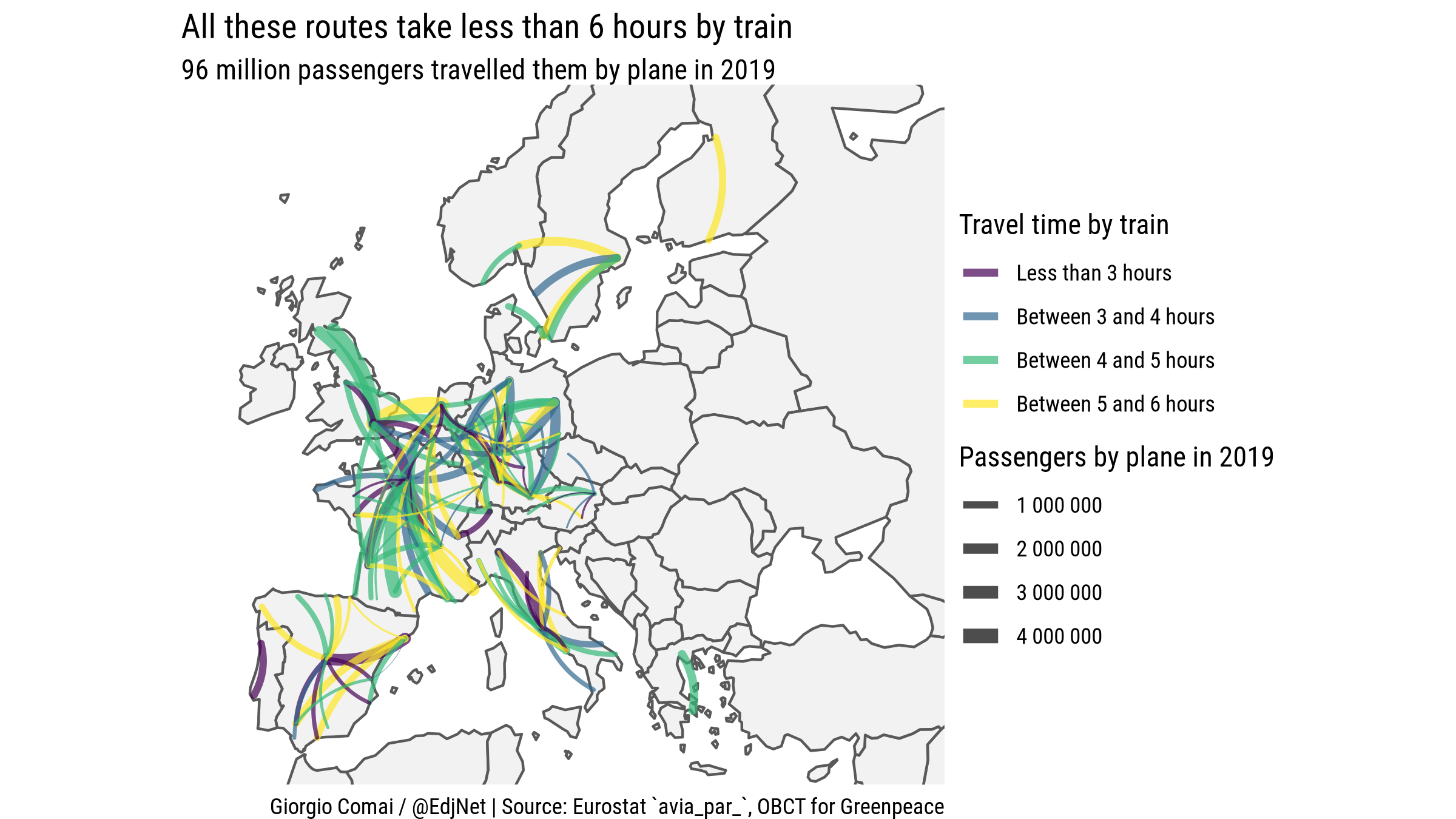
Here’s a few alternative versions of this map based on a routes involving a single country:

routes_by_country_f <- function(country, country_label,
                                xlimits = c(-12, 40),
                                ylimits = c(36, 66)) {
   
  current_country_df <- passengers_less_than_6h_df %>% 
    dplyr::filter(stringr::str_detect(string = `Connected countries`, pattern = country))
  
  total_passengers_n <- current_country_df %>% 
  summarise(passengers= sum(`Passengers by plane in 2019`)) %>% 
  pull(passengers)
  
routes_map_current_country_gg <- ggplot2::ggplot(data = current_country_df) +
  ggplot2::geom_sf(data = world_sf %>% filter(NAME_ENGL!="Iceland"), fill = "grey95") +
  ggplot2::scale_x_continuous(name = "", limits = xlimits) +
  ggplot2::scale_y_continuous(name = "", limits = ylimits) +
  geom_curve(
    aes(
      x = origin_longitude, y = origin_latitude,
      xend = destination_longitude, yend = destination_latitude,
      color = `Travel time by train`,
      size = `Passengers by plane in 2019`
    ),
    curvature = 0.2,
    alpha = 0.7,
    lineend = "round"
  ) +
  ggplot2::theme_void() +
  scale_color_viridis_d() +
  scale_size(labels = scales::number, range = c(0.1, 3)) +
  labs(title = paste("All these routes involving", country_label, "take less than 6 hours by train"),
       subtitle = paste(round(total_passengers_n/1E6), "million passengers travelled them by plane in 2019"), 
       caption = "Giorgio Comai / @EdjNet | Source: Eurostat `avia_par_`, OBCT for Greenpeace") +
theme(text = element_text(family = "Roboto Condensed"),
      plot.title = element_text(),
      plot.subtitle = element_text()) +
  guides(color = guide_legend(override.aes = list(size = 1.5), order = 1))



ggsave(plot = routes_map_current_country_gg, 
       filename = fs::path("maps", paste0("routes_map_", country, "_gg.png")),
       width = 8,
       height = 4.5,
       bg = "white")
routes_map_current_country_gg
}

routes_by_country_f(country = "UK", country_label = "the United Kingdom",
                    xlimits = c(-11, 20),
                    ylimits = c(42, 60))

routes_by_country_f(country = "IT", country_label = "Italy",
                    xlimits = c(-5, 25),
                    ylimits = c(35, 50))

routes_by_country_f(country = "DE", country_label = "Germany",
                    xlimits = c(-5, 25),
                    ylimits = c(46, 56 )) 

routes_by_country_f(country = "ES", country_label = "Spain",
                    xlimits = c(-15, 10),
                    ylimits = c(35, 47)) 

routes_by_country_f(country = "FR", country_label = "France",
                    xlimits = c(-8, 13),
                    ylimits = c(42, 55))

routes_by_country_f(country = "BE", country_label = "Belgium",
                   xlimits = c(-8, 15),
                    ylimits = c(43, 55)) 

routes_by_country_f(country = "NL", country_label = "the Netherlands",
                    xlimits = c(-8, 15),
                    ylimits = c(43, 55))

If you want to explore the data further. An interactive table with all flights included in the dataset:

library("crosstalk")
library("reactable")

data <- SharedData$new(european_hub_land_routes_df %>%
  transmute(ranking, route, passengers, distance_km = round(distance_km)))

bscols(
  widths = c(3, 9),
  list(
    #  filter_checkbox("type", "Type", data, ~type),
    filter_slider("passengers", "Passengers", data, ~passengers, width = "100%"),
    filter_slider("distance_km", "Distance", data, ~distance_km, width = "100%")
    # ,
    # filter_select("route", "Route", data, ~route)
    # ,
    # filter_select("origin_airport_country", "Country of departure", data, ~origin_airport_country)
  ),
  reactable(data, minRows = 10)
)

Passengers

Distance

library("crosstalk")
library("reactable")

data <- SharedData$new(train_routes_coords_df %>%
  #  dplyr::filter(stringr::str_detect(string = `Connected countries`, pattern = "IT")) %>%
  group_by(route_qid) %>%
  mutate(hours_by_train = (min(`Duration of trips (2019)`) %>% as.numeric()) / 3600) %>%
  ungroup() %>%
  distinct(route_qid, .keep_all = TRUE) %>%
  arrange(desc(passengers)) %>%
  transmute(
    ranking = row_number(),
    type = `Type of connection`,
    countries = `Connected countries`,
    route = Connection,
    passengers,
    hours_by_train = round(hours_by_train, digits = 2),
    distance_km = round(Distance)
  ))

bscols(
  widths = c(3, 9),
  list(
    filter_checkbox("type", "Type", data, ~type),
    filter_slider("passengers", "Passengers", data, ~passengers, width = "100%"),
    filter_slider("distance_km", "Distance", data, ~distance_km, width = "100%"),
    filter_slider("hours_by_train", "Hours by train", data, ~hours_by_train, width = "100%"),
    filter_select("route", "Route", data, ~route),
    filter_select("countries", "Countries", data, ~countries)
  ),
  reactable(data, minRows = 10)
)

Type

domestic

domestic non-EU

extra-EU

international

Passengers

Distance

Hours by train

Route

Countries

Summary of datasets available for download and main data issues

If you’ve gone through the whole document, you already know that, but just in case: data for CZ, BA, AL, MD, and XK have been added based on arrivals as recorded on receiving sides of these flights; domestic flights or flights between them would not appear

• european_routes_ranking.csv: 3 889 rows, 13 columns: ‘ranking’, ‘type’, ‘route_code’, ‘passengers’, ‘route_name’, ‘origin_airport_code’, ‘origin_airport_country’, ‘origin_airport_icao’, ‘origin_airport_name’, ‘destination_airport_code’, ‘destination_airport_country’, ‘destination_airport_icao’, and ‘destination_airport_name’
• european_routes_ranking_with_turkey.csv: same as above, but including data from Turkey
• airport_qid_icao_details.csv: this is a dataset with details on all items with an ICAO code in Wikidata across the world, completely based on Wikidata, and used for matching (be mindful about duplicates and potential data issues in particular with minor airfields): 20 255 rows, 16 columns: ‘airport_qid’, ‘airport’, ‘country_qid’, ‘country’, ‘administrative_entity_qid’, ‘administrative_entity’, ‘latitude’, ‘longitude’, ‘iata_code’, ‘icao_code’, ‘hub_qid’, ‘hub’, ‘hub_latitude’, ‘hub_longitude’, ‘replaced_by_qid’, and ‘replaced_by_icao_code’
• airport_qid_unique_icao_details.csv: same as above, but without duplicates, and probably more suitable for most use cases: 19 932 rows, 16 columns: ‘airport_qid’, ‘airport’, ‘country_qid’, ‘country’, ‘administrative_entity_qid’, ‘administrative_entity’, ‘latitude’, ‘longitude’, ‘iata_code’, ‘icao_code’, ‘hub_qid’, ‘hub’, ‘hub_latitude’, ‘hub_longitude’, ‘replaced_by_qid’, and ‘replaced_by_icao_code’
• european_airports_with_wikidata_details.csv: dataset with details on all airports that actually appear in Eurostat’s avia_par_ datasets. All of them have a set of coordinates: 429 rows, 15 columns: ‘country’, ‘icao_code’, ‘airport_qid’, ‘airport’, ‘country_qid’, ‘country_name’, ‘administrative_entity_qid’, ‘administrative_entity’, ‘latitude’, ‘longitude’, ‘iata_code’, ‘hub_qid’, ‘hub’, ‘hub_latitude’, and ‘hub_longitude’
• european_airports_with_wikidata_details_fixed_hubs.csv: similar to the above, but now each row also has a “hub”, i.e. the main city or location served by the airport, with relevant coordinates and Wikidata identifier. 429 rows, 15 columns: ‘country’, ‘icao_code’, ‘airport_qid’, ‘airport’, ‘country_qid’, ‘country_name’, ‘administrative_entity_qid’, ‘administrative_entity’, ‘latitude’, ‘longitude’, ‘iata_code’, ‘hub_qid’, ‘hub’, ‘hub_latitude’, and ‘hub_longitude’
• european_hub_routes.csv: dataset with all European flights routes merged by hub (e.g. all London airports are summed together as a single destination). 3 318 rows, 12 columns: ‘ranking’, ‘route’, ‘passengers’, ‘origin_hub’, ‘origin_hub_qid’, ‘origin_hub_latitude’, ‘origin_hub_longitude’, ‘destination_hub’, ‘destination_hub_qid’, ‘destination_hub_latitude’, ‘destination_hub_longitude’, and ‘distance_km’
• european_hub_land_routes.csv: similar to the above, but only routes that can plausibly be travelled by land are included. 2 345 rows, 12 columns: ‘ranking’, ‘route’, ‘passengers’, ‘distance_km’, ‘origin_hub’, ‘origin_hub_qid’, ‘origin_hub_latitude’, ‘origin_hub_longitude’, ‘destination_hub’, ‘destination_hub_qid’, ‘destination_hub_latitude’, and ‘destination_hub_longitude’
• train_routes.csv. This is the original dataset produced by OBC Transeuropa for Greenpeace. 575 rows, 22 columns: ‘ID’, ‘top 150 intra-EU routes’, ‘top 250 European routes’, ‘Type of connection’, ‘Connected countries’, ‘N. of air passengers (2019)’, ‘Connection’, ‘Origin’, ‘Destination’, ‘via’, ‘N. of transfers (2019)’, ‘Is a night train involved? (2019)’, ‘Time of departure (2019)’, ‘Time of arrival (2019)’, ‘Duration of day trips (2019)’, ‘Duration of trips involving night trains (2019)’, ‘Duration of trips (2019)’, ‘Distance’, ‘Average speed of the journey (2019)’, ‘N. of weekly direct connections (2019)’, ‘Shortest duration in 2021’, and ‘Notes’
• train_routes_coords.csv. Same as above, but with matching coordinates for the arrival and departure, distance, and unique identifiers that enables matching with previous datasets listed here or getting more data from Wikidata. 584 rows, 32 columns: ‘ID’, ‘top 150 intra-EU routes’, ‘top 250 European routes’, ‘Type of connection’, ‘Connected countries’, ‘N. of air passengers (2019)’, ‘Connection’, ‘Origin’, ‘Destination’, ‘via’, ‘N. of transfers (2019)’, ‘Is a night train involved? (2019)’, ‘Time of departure (2019)’, ‘Time of arrival (2019)’, ‘Duration of day trips (2019)’, ‘Duration of trips involving night trains (2019)’, ‘Duration of trips (2019)’, ‘Distance’, ‘Average speed of the journey (2019)’, ‘N. of weekly direct connections (2019)’, ‘Shortest duration in 2021’, ‘Notes’, ‘origin_hub_qid’, ‘origin_latitude’, ‘origin_longitude’, ‘destination_hub_qid’, ‘destination_latitude’, ‘destination_longitude’, ‘distance_air_km’, ‘distance_difference_km’, ‘route_qid’, and ‘passengers’

License

This repository and related dataset is distributed under a Creative Commons CC BY license.

The dataset on trains has been produced by OBC Transeuropa for Greenpeace. Read the full report, or check out this article by Lorenzo Ferrari and Gianluca De Feo for context.

Data on flights have been distributed by Eurostat. See the avia_par_ dataset for licensing and more details.

Code and datasets in this repository are by Giorgio Comai/OBCT/EDJNet.

---

1. Kosovo is usually marked separately in other maps distributed by the EU, including those with NUTS regions, but not in its world map: https://gisco-services.ec.europa.eu/distribution/v2/countries/download/↩︎